Copy of chapter 03

Chapter 3

VECTOR CALCULUS
No man really becomes a fool until he stops asking questions.
—CHARLES P. STEINMETZ

3.1 INTRODUCTION

Chapter 1 is mainly on vector addition, subtraction, and multiplication in Cartesian coordi-
nates, and Chapter 2 extends all these to other coordinate systems. This chapter deals with
vector calculus—integration and differentiation of vectors.
The concepts introduced in this chapter provide a convenient language for expressing
certain fundamental ideas in electromagnetics or mathematics in general. A student may
feel uneasy about these concepts at first—not seeing "what good" they are. Such a student
is advised to concentrate simply on learning the mathematical techniques and to wait for
their applications in subsequent chapters.

J.2 DIFFERENTIAL LENGTH, AREA, AND VOLUME

Differential elements in length, area, and volume are useful in vector calculus. They are
defined in the Cartesian, cylindrical, and spherical coordinate systems.

A. Cartesian Coordinates
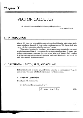
From Figure 3.1, we notice that

(1) Differential displacement is given by

d = dx ax + dy ay + dz az (3.1)

53

54 Vector Calculus

Figure 3.1 Differential elements in the
right-handed Cartesian coordinate system.

•A-

(2) Differential normal area is given by

dS = dy dz a*
dxdz av (3.2)
dzdy a,

and illustrated in Figure 3.2.
(3) Differential volume is given by

dv = dx dy dz (3.3)

dy iaz

dz <

a^ dy

(a) (b) (c)

Figure 3.2 Differential normal areas in Cartesian coordinates:
(a) dS = dy dz a^, (b) dS = dxdz ay, (c) dS = dx dy a,

3.2 DIFFERENTIAL LENGTH, AREA, AND VOLUME 55

These differential elements are very important as they will be referred to again and
again throughout the book. The student is encouraged not to memorize them, however, but
to learn to derive them from Figure 3.1. Notice from eqs. (3.1) to (3.3) that d and dS are
vectors whereas dv is a scalar. Observe from Figure 3.1 that if we move from point P to Q
(or Q to P), for example, d = dy ay because we are moving in the y-direction and if we
move from Q to S (or S to Q), d = dy ay + dz az because we have to move dy along y, dz
along z, and dx = 0 (no movement along x). Similarly, to move from D to Q would mean
that dl = dxax + dyay + dz az.
The way dS is denned is important. The differential surface (or area) element dS may
generally be defined as
dS = dSan (3.4)

where dS is the area of the surface element and an is a unit vector normal to the surface dS
(and directed away from the volume if dS is part of the surface describing a volume). If we
consider surface ABCD in Figure 3.1, for example, dS = dydzax whereas for surface
PQRS, dS = -dy dz ax because an = -ax is normal to PQRS.
What we have to remember at all times about differential elements is d and how to
get dS and dv from it. Once d is remembered, dS and dv can easily be found. For example,
dS along ax can be obtained from d in eq. (3.1) by multiplying the components of d along
a^, and az; that is, dy dz ax. Similarly, dS along az is the product of the components of d
along ax and ay; that is dx dy az. Also, dv can be obtained from d as the product of the three
components of dl; that is, dx dy dz. The idea developed here for Cartesian coordinates will
now be extended to other coordinate systems.

B. Cylindrical Coordinates
Notice from Figure 3.3 that in cylindrical coordinates, differential elements can be found
as follows:

(1) Differential displacement is given by

dl = dpap + p dcj> a 0 + dz a z (3.5)

(2) Differential normal area is given by

dS = p d<j> dz ap
dp dz a^ (3.6)
p d4> dp az

(3) Differential volume is given by

dv = p dp dcf> dz (3.7)

56 Vector Calculus

Figure 3.3 Differential elements in
cylindrical coordinates.
dp
1

-dz

z
pd<t>

As mentioned in the previous section on Cartesian coordinates, we only need to re-
member dl; dS and dv can easily be obtained from dl. For example, dS along az is the
product of the components of dl along ap and a^; that is, dp p d<f> az. Also dv is the product
of the three components of dl; that is, dp p d<j> dz.

C. Spherical Coordinates
From Figure 3.5, we notice that in spherical coordinates,

(1) The differential displacement is

dl = drar + rdd ae + r sin 0 d<f> a 0 (3.8)

(b) (c)

~-y

Figure 3.4 Differential normal areas in cylindrical coordinates:
(a) dS = pd<j> dz ap, (b) dS = dp dz a^, (c) dS = p d<f> dp az

3.2 DIFFERENTIAL LENGTH, AREA, AND VOLUME 57

Figure 3.5 Differential elements
in the spherical coordinate system.

pd<(> = r s i n 6 d<j>

(2) The differential normal area is

dS = r2 sin 6 d6 d<f> a r
r sin 6 dr d<j> a# (3.9)
r dr dd aA

(3) The differential volume is

dv = r2 sind drdd. (3.10)

r sin 0,1 •'' r sin 6dcf>
ar

/ /dr
r,in '
ae r
(a) (b) (c)

w.

Figure 3.6 Differential normal areas in spherical coordinates:
(a) dS = r2 sin 0 dO d<j> ar, (b) dS = r sin 0 dr d<j> a^,
(c) dS = rdr dd a^,

58 Vector Calculus

Again, we need to remember only dl from which dS and dv are easily obtained. For
example, dS along ae is obtained as the product of the components of dl along a r and
a^; that is, dr • r sin 6 d4>; dv is the product of the three components of dl; that is,
dr • r dd • r sin 6 d<t>.

Consider the object shown in Figure 3.7. Calculate
EXAMPLE 3.1
(a) The distance BC
(b) The distance CD
(c) The surface area ABCD
(d) The surface area ABO
(e) The surface area A OFD
(f) The volume ABDCFO

Solution:
Although points A, B, C, and D are given in Cartesian coordinates, it is obvious that the
object has cylindrical symmetry. Hence, we solve the problem in cylindrical coordinates.
The points are transformed from Cartesian to cylindrical coordinates as follows:

A(5,0,0)-»A(5,0°,0)

5(0, 5, 0) -» 5( 5, - , 0

C(0, 5, 10) -» C( 5, - , 10

D(5,0, 10)-»£>(5,0°, 10)

Figure 3.7 For Example 3.1.

C(0, 5, 10)
0(5, 0, 10)

5(0,5,0)

3.2 DIFFERENTIAL LENGTH, AREA, AND VOLUME • 59

(a) Along BC, dl = dz; hence,

BC = | dl= dz= 10

(b) Along CD, dl = pd<f> and p = 5, so
CTSIl ir/2
CD= p d<j) = 5 = 2.5TT

(c) For ABCD, dS = pd<t> dz, p = 5. Hence,
ir/2 r 10 x/2 r10

area ABCD = dS = I pd =5 = 25TT

(d) For ABO, dS = pd<j> dp and z = 0, so
TTr/2 r5 (-TT/2 (-5

p dcj> dp = d<j> p dp = 6.25TT

(e) For AOFD, d5 = dp dz and 0 = 0°, so

area AOFD = dp dz = 50

(f) For volume ABDCFO, dv = pd<f> dz dp. Hence,
r5 rir/2 rlO <• 10 /-ir/2 <-5
v = L/ v = p d0 dz dp = dz J = 62.5TT

PRACTICE EXERCISE 3.1

Refer to Figure 3.26; disregard the differential lengths and imagine that the object is
part of a spherical shell. It may be described as 3 S r < 5 , 60° < 0 < 90°,
45° < 4> < 60° where surface r = 3 is the same as AEHD, surface 0 = 60° is A£FB,
and surface < = 45° is AfiCO. Calculate
£
(a) The distance DH
(b) The distance FG
(c) The surface area AEHD
(d) The surface area ABDC
(e) The volume of the object

Answer: (a) 0.7854, (b) 2.618, (c) 1.179, (d) 4.189, (e) 4.276.

60 Vector Calculus

3.3 LINE, SURFACE, AND VOLUME INTEGRALS

The familiar concept of integration will now be extended to cases when the integrand in-
volves a vector. By a line we mean the path along a curve in space. We shall use terms such
as line, curve, and contour interchangeably.

The line integral A • d is the integral of ihc tangential component of A along
curve L.

Given a vector field A and a curve L, we define the integral
fb
A-dl = (3.11)

as the line integral of A around L (see Figure 3.8). If the path of integration is a closed
curve such as abca in Figure 3.8, eq. (3.11) becomes a closed contour integral

A-dl (3.12)

which is called the circulation of A around L.
Given a vector field A, continuous in a region containing the smooth surface S, we
define the surface integral or the^wx of A through S (see Figure 3.9) as

= A cos OdS= A-andS

or simply

(3.13)

Figure 3.8 Path of integration of vector field A.

pathi

3.3 LINE, SURFACE, AND VOLUME INTEGRALS 61

Figure 3.9 The flux of a vector field A
through surface S.
surface S

where, at any point on S, an is the unit normal to S. For a closed surface (defining a
volume), eq. (3.13) becomes

= * A • dS (3.14)
•'s

which is referred to as the net outward flux of'A from S. Notice that a closed path defines
an open surface whereas a closed surface defines a volume (see Figures 3.11 and 3.16).
We define the integral

(3.15)

as the volume integral of the scalar pv over the volume v. The physical meaning of a line,
surface, or volume integral depends on the nature of the physical quantity represented by
A or pv. Note that d, dS, and dv are all as defined in Section 3.2.

Given that F = x2ax - xz&y - y2&z, calculate the circulation of F around the (closed) path
shown in Figure 3.10.

Solution:
The circulation of F around path L is given by

Fdl = + + + ) F • d
h h V
where the path is broken into segments numbered 1 to 4 as shown in Figure 3.10.
For segment 1, v = 0 = z
= jc 2 a x , = dxax
Notice that d is always taken as along +a x so that the direction on segment 1 is taken care
of by the limits of integration. Thus,

¥-d= x2dx = -

62 • Vector Calculus


*-y

For segment 2, x = 0 = z, F = -y 2 a z , d = dy ay, F • d = 0. Hence,

F • dl = 0

For segment 3, y = 1, F = x2ax - xz&y - az, and dl = dxax + dz a2, so

F • d = (xldx - dz)

But on 3, z = *; that is, Jx = dz. Hence,
-l
F • d = (xz - 1) dx = — - x
3
3 '

For segment 4, x = 1, so F = ax — zay — y2az, and d = dy ay + dz az. Hence,

Fdl = (-zrfy-/dz)

But on 4, z = y; that is, dz =rfy,so

0 2 3
°=5
F • d =
.4 J, 1 6

By putting all these together, we obtain

3.4 DEL OPERATOR 63

Figure 3.11 For Practice Exercise 3.2.


Calculate the circulation of
A = p cos <j> ap + z sin $ a2
around the edge L of the wedge defined by 0 £ 60°, z = 0 and
shown in Figure 3.11.

Answer: 1.

3.4 DEL OPERATOR

The del operator, written V, is the vector differential operator. In Cartesian coordinates,

V = a + (3.16)
-dx'* Tya> +
Tza<

This vector differential operator, otherwise known as the gradient operator, is not a vector
in itself, but when it operates on a scalar function, for example, a vector ensues. The oper-
ator is useful in denning

1. The gradient of a scalar V, written, as W
2. The divergence of a vector A, written as V • A
3. The curl of a vector A, written as V X A
4. The Laplacian of a scalar V, written as V V

Each of these will be denned in detail in the subsequent sections. Before we do that, it
is appropriate to obtain expressions for the del operator V in cylindrical and spherical
coordinates. This is easily done by using the transformation formulas of Section 2.3
and 2.4.

64 Vector Calculus

To obtain V in terms of p, <j>, and z, we recall from eq. (2.7) that 1

tan 0 = —
x

Hence

sin (j) d
— = cos q> (3.17)
dx dp p dq>

d d COS 4> d
— = sin <f> 1 (3.18)
dy dp p 8<t>

Substituting eqs. (3.17) and (3.18) into eq. (3.16) and making use of eq. (2.9), we obtain V
in cylindrical coordinates as

d ] d d
V = 3 -f- 3 — -a (3.19)
" dp P d = -
x

to obtain
d d cos 6 cos 4> d sin <j> d
— = sin 6 cos cp 1 (3.20)
dx dr r 30 p dcp
8 . d cos 0 sin 0 3 cos 0 5
— = sin 0 sin 

d d sin 0 d
— = cos 6 (3.22)
dz dr r 80

Substituting eqs. (3.20) to (3.22) into eq. (3.16) and using eq. (2.23) results in V in spheri-
cal coordinates:

1 d 1
(3.23)

Notice that in eqs. (3.19) and (3.23), the unit vectors are placed to the right of the differen-
tial operators because the unit vectors depend on the angles.

'A more general way of deriving V, V • A, V X A, W, and V2V is using the curvilinear coordinates.
See, for example, M. R. Spiegel, Vector Analysis and an Introduction to Tensor Analysis. New York:
McGraw-Hill, 1959, pp. 135-165.

3.5 GRADIENT OF A SCALAR 65

3.5 GRADIENT OF A SCALAR

The gradient of a scalar field V is a vccior thai represents both the magnitude and the
direction of the maximum space rale of increase of V.

A mathematical expression for the gradient can be obtained by evaluating the difference in
the field dV between points Pl and P2 of Figure 3.12 where V,, V2, and V3 are contours on
which V is constant. From calculus,
dV dV dV
= — dx + — dy + — dz
dx dy dz
(3.24)
dV dV dV ,
ax + — ay + — az) • (dx ax + dy ay + dz az)
y +

For convenience, let

dV dV dV
—*x + ~ay
dx By + dz
— (3.25)

Then

dV = G • d = G cos 6 dl

or
dV
— = Gcos6 (3.26)
dl

Figure 3.12 Gradient of a scalar.

*- y

66 Vector Calculus

where d is the differential displacement from P, to P2 and 6 is the angle between G and d.
From eq. (3.26), we notice that dV/dl is a maximum when 0 = 0, that is, when d is in the
direction of G. Hence,
dV
(3.27)
dl dn
where dV/dn is the normal derivative. Thus G has its magnitude and direction as those of
the maximum rate of change of V. By definition, G is the gradient of V. Therefore:
dV 3V dV
grad V = W = — ax + — ay + — a,
s v (3.28)
5x dy dz
By using eq. (3.28) in conjunction with eqs. (3.16), (3.19), and (3.23), the gradient of
V can be expressed in Cartesian, cylindrical, and spherical coordinates. For Cartesian co-
ordinates

dV dV dV
Vy = — a, - ay -
v a.
dx ay dz '

for cylindrical coordinates,

dV i dV dV
vy = — a<4 -1 a. (3.29)
dp 3(f> * dz

and for spherical coordinates,

av i ay 1 ay
= — ar + a« + (3.30)
dr r 39 rsinfl d<f>

The following computation formulas on gradient, which are easily proved, should be
noted:
(a) V(v + u) = vy + vu (3.31a)
(b) V{vu) = yvt/ + uw (3.31b)
- yvc/
(c) (3.31c)

(d) " = nVn~xVV (3.31d)
where U and V are scalars and n is an integer.
Also take note of the following fundamental properties of the gradient of a scalar
field V:

1. The magnitude of Vy equals the maximum rate of change in V per unit distance.
2. Vy points in the direction of the maximum rate of change in V.
3. Vy at any point is perpendicular to the constant V surface that passes through that
point (see points P and Q in Figure 3.12).

3.5 GRADIENT OF A SCALAR 67

4. The projection (or component) of VV in the direction of a unit vector a is W • a
and is called the directional derivative of V along a. This is the rate of change of V
in the direction of a. For example, dV/dl in eq. (3.26) is the directional derivative of
V along PiP2 in Figure 3.12. Thus the gradient of a scalar function V provides us
with both the direction in which V changes most rapidly and the magnitude of the
maximum directional derivative of V.
5. If A = VV, V is said to be the scalar potential of A.

Find the gradient of the following scalar fields:
EXAMPLE 3.3
(a) V = e~z sin 2x cosh y
(b) U = p2z cos 2<t>
(c) W= lOrsin20cos<£

Solution:
dv_t dV dV
(a)
dx'
= 2e zcos 2x cosh y ax + e zsin 2x sinh y ay — e Jsin 2x cosh y az

v™-¥ 1 dU
P d0
dU_
a
dz 7
= 2pz cos 2<f> ap — 2pz sin 2(/> a^ + p cos 20 az
_ aw i aw i aw
dr a r 36 " rsinfl 90 "
= 10 sin2 6 cos 0 a r + 10 sin 26 cos 0 a# — 10 sin 0 sin 01


Determine the gradient of the following scalar fields:
(a) U = x2y + xyz
(b) V = pz sin <t> + z2 cos2 <t> + p2
(c) / = cos 6 sin 0 In r + r2<j>

Answer: (a) y{2x + z)ax + x(x + z)ay + xyaz

(b) (z sin 0 + 2p)ap + (z cos 0 sin
(p sin <t> + 2z c o s 2 <j>)az
/cos 0 sin In r + r cosec 0

68 i Vector Calculus

Given W = x2y2 + xyz, compute VW and the direction derivative dW/dl in the direction
EXAMPLE 3.4
3ax + 4ay + 12az at (2,-1,0).

dW dW dW
Solution: VW = a, +
x av +
y a,
dx dy dz z
= (2xyz + yz)ax + (2xzy + xz)ay + (xy)az
At (2, -1,0): VW = ay - 2az
Hence,


Given <P = xy + yz + xz, find gradient 0 at point (1,2, 3) and the directional deriv-
ative of <P at the same point in the direction toward point (3,4,4).

Answer: 5ax + 4a.. + 3az, 7.

Find the angle at which line x = y = 2z intersects the ellipsoid x2 + y2 + 2z2 = 10.
EXAMPLE 3.5

Solution:
Let the line and the ellipsoid meet at angle j/ as shown in Figure 3.13. The line x = y = 2z
can be represented by
r(X) = 2Xa^ + 2X3,, + Xaz
where X is a parameter. Where the line and the ellipsoid meet,
(2X)2 + (2X)2 + 2X2 = 10 ~> X = ± 1
Taking X = 1 (for the moment), the point of intersection is (x, y, z) = (2,2,1). At this
point, r = 2a^ + 2a,, + az.

Figure 3.13 For Example 3.5; plane of intersection of a line
with an ellipsoid.
ellipsoid
/

3.6 DIVERGENCE OF A VECTOR AND DIVERGENCE THEOREM 69

The surface of the ellipsoid is defined by
f(x,y,z)=x2 + y2 + 2z2-W
The gradient of/is
Vf=2xax + 2yay + 4zaz
At (2,2,1), V/ = 4ax + 4ay + 4a r Hence, a unit vector normal to the ellipsoid at the point
of intersection is
v
. _^ / _ a. + a. + a,
V3

Taking the positive sign (for the moment), the angle between an and r is given by
an • r 2+ 2+ 1
cos 6 = = «n p
•r VW9 3V3
Hence, j/ = 74.21°. Because we had choices of + or — for X and an, there are actually four
possible angles, given by sin i/< = ±5/(3 V3).


Calculate the angle between the normals to the surfaces x y + z — 3 and
x log z — y2 = - 4 at the point of intersection ( 1, 2,1).
—

Answer: 73.4°.

3.6 DIVERGENCE OF A VECTOR AND DIVERGENCE
THEOREM

From Section 3.3, we have noticed that the net outflow of the flux of a vector field A from
a closed surface S is obtained from the integral § A • dS. We now define the divergence of
A as the net outward flow of flux per unit volume over a closed incremental surface.

The divergence of A at a given point P is ihc outward (lux per unii volume as the
volume shrinks about P.

Hence,

A-dS
div A = V • A = lim (3.32)
Av—>0 Av

70 Vector Calculus

• P

(a) (b) (c)

Figure 3.14 Illustration of the divergence of a vector field at P; (a) positive
divergence, (b) negative divergence, (c) zero divergence.

where Av is the volume enclosed by the closed surface S in which P is located. Physically,
we may regard the divergence of the vector field A at a given point as a measure of how
much the field diverges or emanates from that point. Figure 3.14(a) shows that the diver-
gence of a vector field at point P is positive because the vector diverges (or spreads out) at
P. In Figure 3.14(b) a vector field has negative divergence (or convergence) at P, and in
Figure 3.14(c) a vector field has zero divergence at P. The divergence of a vector field can
also be viewed as simply the limit of the field's source strength per unit volume (or source
density); it is positive at a source point in the field, and negative at a sink point, or zero
where there is neither sink nor source.
We can obtain an expression for V • A in Cartesian coordinates from the definition in
eq. (3.32). Suppose we wish to evaluate the divergence of a vector field A at point
P(xo,yo, zo); we let the point be enclosed by a differential volume as in Figure 3.15. The
surface integral in eq. (3.32) is obtained from

A • dS = M + + + + + ) A • dS (3.33)
S ^ •'front •'back •'left ^right Aop •'bottorr/

A three-dimensional Taylor series expansion of Ax about P is

BAr
Ax(x, v, z) = Ax(xo, yo, Zo) **„) + (y-yo)
dy
dx (3.34)
+ (z - Zo)— + higher-order terms
dz

For the front side, x = xo + dx/2 and dS = dy dz ax. Then,

dx dA
A • dS = dy dz xo, yo, zo) + — + higher-order terms
front
2 dx

For the back side, x = x0 - dx/2, dS - dy dz(~ax). Then,

dx dA
A • dS = -dydzl Ax(x0, yo, zo) ~ higher-order terms
L
L
2 dx
back

3.6 DIVERGENCE OF A VECTOR AND DIVERGENCE THEOREM 71

Figure 3.15 Evaluation of V • A at point
P(x0, Jo. Zo).
top side

dz
front — - i •/»
side

dy
Jx
+. right side

Hence,

dA
A • dS + I A • dS = dx dy dz — - + higher-order terms (3.35)
•'front -"back dx

By taking similar steps, we obtain

dAy
A • dS + A-dS = dxdydz + higher-order terms (3.36)
left right dy

and

A-dS A • dS = dx dy dz — + higher-order terms (3.37)
•"top ^bottom dz
Substituting eqs. (3.35) to (3.37) into eq. (3.33) and noting that Av = dx dy dz, we get

• $s, A • dS Mi (3.38)
AV->O Av dz
because the higher-order terms will vanish as Av — 0. Thus, the divergence of A at point
>
P(xo, yo, zo) in a Cartesian system is given by

(3.39)

Similar expressions for V • A in other coordinate systems can be obtained directly
from eq. (3.32) or by transforming eq. (3.39) into the appropriate coordinate system. In
cylindrical coordinates, substituting eqs. (2.15), (3.17), and (3.18) into eq. (3.39) yields

1 dA6 dA,
V-A
P dp
f+ (3.40)

72 Vector Calculus

Substituting eqs. (2.28) and (3.20) to (3.22) into eq. (3.39), we obtain the divergence of A
in spherical coordinates as

1 d 2 1 1
V- A - .e sin 0) H (3.41)
dr(' A
r sin i rsind d<f>

Note the following properties of the divergence of a vector field:

1. It produces a scalar field (because scalar product is involved).
2. The divergence of a scalar V, div V, makes no sense.
3. V • (A + B) = V • A + V • B
4. V • (VA) = VV • A + A • VV

From the definition of the divergence of A in eq. (3.32), it is not difficult to expect that

(3.42)

This is called the divergence theorem, otherwise known as the Gauss-Ostrogradsky
theorem.

Hie divergence theorem stales thai Ihe total mil ward llux of a vector licld A through
ihc closed surface." . is ihe same as the volume integral of the divergence of A.
V

To prove the divergence theorem, subdivide volume v into a large number of small
cells. If the Mi cell has volume Avk and is bounded by surface Sk

A-dS
Avt (3.43)

Since the outward flux to one cell is inward to some neighboring cells, there is cancellation
on every interior surface, so the sum of the surface integrals over Sk's is the same as the
surface integral over the surface 5. Taking the limit of the right-hand side of eq. (3.43) and
incorporating eq. (3.32) gives

A-dS= V-Adv (3.44)

which is the divergence theorem. The theorem applies to any volume v bounded by the
closed surface S such as that shown in Figure 3.16 provided that A and V • A are continu-

3.6 DIVERGENCE OF A VECTOR AND DIVERGENCE THEOREM M 73

Figure 3.16 Volume v enclosed by surface S.

Volume v •
. Closed Surface S

ous in the region. With a little experience, it will soon become apparent that volume inte-
grals are easier to evaluate than surface integrals. For this reason, to determine thefluxof
A through a closed surface we simply find the right-hand side of eq. (3.42) instead of the
left-hand side of the equation.

Determine the divergence of these vector fields:
EXAMPLE 3.6
(a) P = x2yz ax + xz az
(b) Q = p sin 0 ap + p2z a$ cos <j) az

(c) T = —z cos d ar + r sin 6 cos <j> a# + cos

Solution:

(a) V • P = —Px + —Pv + —Pz
dx
dx x dy y dz z
= ~(x2yz)
dx dy
= 2xyz + x

(b) V • Q = —^- (pQp) + -~Q^ + ^-Qz
P dp p B(j) dz
d
1 S , 1 d 2
= - — (P sin 0) + - — (p z) + — (z cos <t>)
P dp p d<t> dz
= 2 sin ^ + cos <j>

(c) V • T = 3 - (r2Tr) + - ^~^(Te sin 6)
r dr r sin 8 B6 r sin 9
1 d 1 d o l a
= -^ — (cos 6) +
2
(r sin 9 cos <£) H — (cos 9)
r dr r sin 0 30 r sin 0 dd>

2r sin 0 cos 6 cos <t> + 0

74 Vector Calculus


Determine the divergence of the following vector fields and evaluate them at the
specified points.
(a) A = yz&x + 4xy&y + j a z at (1, - 2 , 3 )
(b) B = pz sin <t> ap + 3pz2 cos <$> a^ at (5, TT/2, 1)
y
(c) C = 2r cos 0 cos <j> ar + r at (1, ir/6, ir/3)

Answer: (a) Ax, 4, (b) (2 - 3z)z sin <f>, - 1 , (c) 6 cos 6 cos <£, 2.598.

If G(r) = lOe 2z(/»aP + a j , determine the flux of G out of the entire surface of the cylinder
EXAMPLE 3.7
p = l , 0 < z < 1. Confirm the result using the divergence theorem.

Solution:
If !P is the flux of G through the given surface, shown in Figure 3.17, then

where ft, Vfc, and Ys are the fluxes through the top, bottom, and sides (curved surface) of
the cylinder as in Figure 3.17.
For Yt,z= ,dS = pdp d<j> az. Hence,

10e > dp d<t>=


J

3.7 CURL OF A VECTOR AND STOKES'S THEOREM 75

For Yb, z = 0 and dS = pdp d<j>(—az). Hence,

G • dS - 10e°pdpd<t> = -10(27r)y

= -107T

For Ys, p = 1, dS = p dz d<j) a Hence,
,.~2z
= I G • dS = | | Kte~ 2z p 2 dz d4> = 10(l) 2 (2ir)
2= 0 J
^) =
-2
= 10TT(1 - e" 2 )

Thus,
- IOTT + 10TT(1 - e~2) = 0

Alternatively, since S is a closed surface, we can apply the divergence theorem:

= <P G-dS = | (V-G)rfv

But

- -
P ap
= - ~ ( p 2 l 0 e ~ 2 z ) - 20e^2z = 0
P dp
showing that G has no source. Hence,

= (V • G) dv = 0


Determine the flux of D = p 2 cos2 0 a^ + z sin 0 a^ over the closed surface of the
cylinder 0 ^ j < I, p = 4. Verify the divergence theorem for this case.

Answer: (Air.

3.7 CURL OF A VECTOR AND STOKES'S THEOREM

In Section 3.3, we defined the circulation of a vector field A around a closed path L as the
integral $LA • d.

76 Vector Calculus

The curl of A is an axial (or rotational) vector whose magnitude is the maximum cir-
culation of A per unit area as the area lends to zero and whose direction is the normal
direction of the area when the area is oriented so as to make the circulation
maximum.''

That is,

A •d
curl A = V X A = lim (3.45)

where the area AS is bounded by the curve L and an is the unit vector normal to the surface
AS and is determined using the right-hand rule.
To obtain an expression for V X A from the definition in eq. (3.45), consider the dif-
ferential area in the ^z-plane as in Figure 3.18. The line integral in eq. (3.45) is obtained as

A • dl = ( + + + jA-dl (3.46)
J
L ^Lb 'be Kd 'dj
We expand the field components in a Taylor series expansion about the center point
P(Xo,yo>zo) as in eq. (3.34) and evaluate eq. (3.46). On side ab, d = dyay and
z = zo - dzli, so

dz
A • d = dy A(xo, yo, zo) ~ — (3.47)
ab
2 dz
On side be, d = dz az and y = yo + dy/2, so

dy dAz
A-dl = dz z(xo, yo, Zo) (3.48)
be
2 dy
On side cd, d = dy ay and z = z0 + dzJ2, so

A • d = -dy | Ay(xo, yo, zo) + y ~j^ (3.49)

Figure 3.18 Contour used in evaluating the ^-component
of V X A at point P(x0, y0, z0).

2
Because of its rotational nature, some authors use rot A instead of curl A.

J

On side da, d = dz Skz and y = yo - dy/2, so

dydAz
A • d = - dz | Az(xo, yo, Zo) ~ — (3.50)
'da
2 dy

Substituting eqs. (3.47) to (3.50) into eq. (3.46) and noting that AS = dy dz, we have

A • d bA7 dAv
lim
AS dy dz

or
dA7 dAy
(curl A)x = (3.51)
By dz

The y- and x-components of the curl of A can be found in the same way. We obtain

dA7
(curl A)y = (3.52a)
dz dx

AAj, dAx
(curl A)z = (3.52b)
dx dy

The definition of V X A in eq. (3.45) is independent of the coordinate system. In
Cartesian coordinates the curl of A is easily found using

VX A = A A A (3.53)
dx dy dz
A A A
nx riy nz

aA z l
VX A =
[dy dx yy
(3.54)
ldAy dAJ
z
[ dx dy J "

By transforming eq. (3.54) using point and vector transformation techniques used in
Chapter 2, we obtain the curl of A in cylindrical coordinates as

ap pa
A A
dp d</>

78 Vector Calculus

or

(3.55)

and in spherical coordinates as

ar r ae r sin 0 a^,
VXA =
~dr ~dd ~d4>
Ar rAe r sin 0 yL

or

V X A
rsinflL 3^ 8<^|ar
(3.56)
l [ 1 dA r 3(M0) ,1 +
iW_M,, a
r [ s i n 0 9(^> ar r ar ae ' "

Note the following properties of the curl:

1. The curl of a vector field is another vector field.
2. The curl of a scalar field V, V X V, makes no sense.
3. V X ( A + B) = V X A + V X B
4. V X (A X B) = A(V • B) - B(V • A) + (B • VA - (A • V)B
5. V X (VA) = VV X A + VV X A
6- The divergence of the curl of a vector field vanishes, that is, V • (V X A) = 0.
7. The curl of the gradient of a scalar field vanishes, that is, V X VV = 0.

Other properties of the curl are in Appendix A.
The physical significance of the curl of a vector field is evident in eq. (3.45); the curl
provides the maximum value of the circulation of the field per unit area (or circulation
density) and indicates the direction along which this maximum value occurs. The curl of a
vector field A at a point P may be regarded as a measure of the circulation or how much the
field curls around P. For example, Figure 3.19(a) shows that the curl of a vector field
around P is directed out of the page. Figure 3.19(b) shows a vector field with zero curl.

Figure 3.19 Illustration of a curl: (a) curl at P points out
of the page; (b) curl at P is zero.

(a) (b)

3.7 CURL OF A VECTOR AND STOKES'S THEOREM • 79

dS Figure 3.20 Determining the sense of d
and dS involved in Stokes's theorem.

Closed Path L

J
Surfaces

Also, from the definition of the curl of A in eq. (3.45), we may expect that

A • d = (VXA)-(iS (3.57)

This is called Stokes's theorem.

Stokes's theorem suites that ihe circulation of a vcclor Meld A around a (closed) pain
/- is equal lo the surface integral ol'lhe curl of A over the open surface S bounded by
/.. (see Figure 3.20) provided that A and V X A are continuous on .V.

The proof of Stokes's theorem is similar to that of the divergence theorem. The surface
S is subdivided into a large number of cells as in Figure 3.21. If the Ath cell has surface area
ASk and is bounded by path Lk.

A-dl
A-dl = A
' d l = ASt (3.58)
AS,

Figure 3.21 Illustration of Stokes's theorem.

80 Vector Calculus

As shown in Figure 3.21, there is cancellation on every interior path, so the sum of the line
integrals around Lk's is the same as the line integral around the bounding curve L. There-
fore, taking the limit of the right-hand side of eq. (3.58) as ASk — 0 and incorporating
>
eq. (3.45) leads to

A • dl = (V X A) • dS

which is Stokes's theorem.
The direction of dl and dS in eq. (3.57) must be chosen using the right-hand rule or
right-handed screw rule. Using the right-hand rule, if we let the fingers point in the direc-
tion ofdl, the thumb will indicate the direction of dS (see Fig. 3.20). Note that whereas the
divergence theorem relates a surface integral to a volume integral, Stokes's theorem relates
a line integral (circulation) to a surface integral.

Determine the curl of the vector fields in Example 3.6.
EXAMPLE 3.8
Solution:
(dPz dPy (dPx dP^ fdPy dPx
(a) V X P = —-* - —*) U + — i - —^ a , + —* a7
V 3j 3z / dz dx J dx dy
= (0 - 0) ax + (x2y - z) (0 - x2z) az
= (x2y - z)ay - x2zaz

= (-y sin 0 - p2) ap + (0 - 0)8* + ^ (3p2z - p cos <t>)az

(z sin <t> + p3)ap + (3pz - cos

(c) V X T = ar
r sin 0 L 30 30
i r i d <

— (cos 0 sin 0) (r sin 0 cos 0) | ar
r sin I 30 30
1 3 (cos0) 3
r sin 0 30 r 2 3r ( r c o s ,
d (COS0)
(r sin 0 cos 0) - —-
dr

(cos 26 + r sin 0 sin 0)a, H— (0 — cos 6)ae
r sin 0
1 / sin (9
+ — 2r sin 0 cos 0 H 2 5-
rV r
/cos 20 . cos 0 / 1
= —r-r + sin 0 I ar + 2 cos 0 + -^ sin 0 a0
Vrsin0 / r

Determine the curl of the vector fields in Practice Exercise 3.6 and evaluate them at
the specified points.

Answer: (a) ax + yay + (4y - z)az, ax - 2% - 1 la,
(b) -6pz cos 0 ap + p sin 0 a^ + (6z - l)z cos 0 a2, 5a,;,
cot 6 I 3
(c) —^ ar - ^2 cot 0 sin 0 + - ^ + 2 sin 6 cos 0 a*,
1.732 ar - 4.5 ae + 0.5 a0.

If A = p cos 0 ap + sin 0 a^, evaluate ^ A • d around the path shown in Figure 3.22.
EXAMPLE 3.9
Confirm this using Stokes's theorem.

Solution:
Let

A-dl + [ + I + I |A-J1
'b 'c 'd

where path L has been divided into segments ab, be, cd, and da as in Figure 3.22.
Along ab, p = 2 and d = p d<t> a0. Hence,
30° 30°
k-d = p sin 0 d(j> = 2(—cos 0) = -(V3 - 1)
= 60° 60°


5

7
/
< L

, C

r
/ ^ t
I ~
/
Xb

0 I 1
is' ^ 1 1 ,

82 H Vector Calculus

Along be, <t> = 30° and d = dp ap. Hence,

2lV3
A • d = p cos <&dp = cos 30° —

Along cd, p = 5 and dl = p d<f> a^. Hence,

60° 60°
p sin <j>d<j> = 5 ( - c o s <f>) = f(V3-0
30°

Along da, <j> = 60° and dl = dp a p . Hence,

21
A • dl = p cos <j>dp = cos 60° —
2
^
Putting all these together results in

5V3 5 21
2 2 4
= — ( V 3 - 1) = 4.941
4

Using Stokes's theorem (because L is a closed path)

A • dl = (V X A)

But dS = pd<(>dpaz and

. 1 3A, I dAo dAz ld dAn
V X A = aj -—^
+ aj —^ - —^ I + a, T | —
dp

= (0 - (0 - p) sin 4> a z

Hence:
60° z-5

(V X A) — (1 + p ) sin <fi p dp d<t>

60° 5
sin i
J
30° 2

= -cos'
27
= — (V3 - 1) = 4.941

3.8 LAPLACIAN OF A SCALAR 83


Use Stokes's theorem to confirm your result in Practice Exercise 3.2.

Answer: 1.

For a vector field A, show explicitly that V • V X A = 0; that is, the divergence of the curl
EXAMPLE 3.10
of any vector field is zero.

Solution:
This vector identity along with the one in Practice Exercise 3.10 is very useful in EM. For
simplicity, assume that A is in Cartesian coordinates.

dx dy dz
dx dy dz A A A

dAz dAy dAy _ dA,
dx' dy' dz dy dz dx dz y dx dy
d fdAz dAy^ d /dAv dA^
dx dy dz V dx2 dz 2 dx 2 dx
d2Az d2Av d Ax AV d A,
dx dy dx dz dy dx dy dz dz dx dz 3y
= 0
d2A7 d2A7
because and so on.
dx dy dy dx


For a scalar field V, show that V X W = 0; that is, the curl of the gradient of any
scalar field vanishes.

Answer: Proof.

.8 LAPLACIAN OF A SCALAR

For practical reasons, it is expedient to introduce a single operator which is the composite
of gradient and divergence operators. This operator is known as the Laplacian.

84 Vector Calculus

The Laplacian of u scalar field V, written as V2V. is the divergence of the gradient
of V.

Thus, in Cartesian coordinates,
Laplacian V = V • W = V2V

d d d dV_
01. OX.. a7 (3.59)
dx' dz' dx ' By'' dz

that is,

(3.60)

Notice that the Laplacian of a scalar field is another scalar field.
The Laplacian of V in other coordinate systems can be obtained from eq. (3.60) by
transformation. In cylindrical coordinates,

(3.61)

and in spherical coordinates,

1 d ( 2dV 1 d f dV 1 d2V
(3.62)
r2 dr dr J r2 sin V ou V dd) ' r2 sin 2 ^ d<j>2

A scalar field V is said to be harmonic in a given region if its Laplacian vanishes in
that region. In other words, if

V2V=0 (3.63)

is satisfied in the region, the solution for V in eq. (3.63) is harmonic (it is of the form of sine
or cosine). Equation (3.63) is called Laplace's equation. Solving this equation will be our
major task in Chapter 6.
We have only considered the Laplacian of a scalar. Since the Laplacian operator V2 is
a scalar operator, it is also possible to define the Laplacian of a vector A. In this context,
V2A should not be viewed as the divergence of the gradient of A, which makes no sense.
Rather, V2A is defined as the gradient of the divergence of A minus the curl of the curl of
A. That is,

V2A = V(V- A) - V X V X A (3.64)

J

3.8 LAPLACIAN OF A SCALAR 85

This equation can be applied in finding V2A in any coordinate system. In the Cartesian
system (and only in that system), eq. (3.64) becomes

V2A = (3.65)

Find the Laplacian of the scalar fields of Example 3.3; that is,
EXAMPLE 3.11
(a) V = e~z sin 2x cosh y
(b) U = p2z cos 20
(c) W = lOr sin2 0 cos 0

Solution:
The Laplacian in the Cartesian system can be found by taking the first derivative and later
the second derivative.
d2V t)2V r)2V

dx 5y dz
= — (2e~z cos 2x cosh y) H (e z
cos 2x sinh y)
dx dy
z
H (~e
sin 2x cosh y)
dz
= -Ae~z sin 2xcoshy + e~z sin 2xcoshy + e~z sin 2xcoshy
= -2e~z sin 2x cosh y
1 d2U d2U
(b)
P dp

= (2p2z cos 20) ~ 4p2z cos 20 + 0
P dp pz
= Az cos 20 — Az cos 20
= 0
1 d ( . ndW d2W
r dr r 2 sin 6 d$ d9 r sin 0 dct>2
2 2

1 r) 1 f)
= -^ — (10r2 sin2 0 cos 0) ; (10r sin 20 sin 6 cos 0)
sin0 d6
lOr sin2 0 cos 0
r 2 sin2 0
2
20 sin 0 cos 0 20r cos 20 sin 6 cos 0
r2 sin 0
lOr sin 26 cos 0 cos 0 10 cos 0
2
r sin 6 r
(2 sin2 0 + 2 cos 20 + 2 cos2 0 - 1 )

( 1 + 2 cos 26)

86 Vector Calculus


Determine the Laplacian of the scalar fields of Practice Exercise 3.3, that is,

(a) V = x2y + xyz
(b) V = pz sin 4> + z2 cos 2 <l> + p2
(c) / = cos 0 sin 4> In r + r 2 <j>

, 2z 2 1
Answer: (a) 2y, (b) 4 + 2 cos 0 5-cos2<^>, (c) —z cos 0 sin <^ (1 - 2 1 n r
cosec 2 $ In r) + 6$.

3.9 CLASSIFICATION OF VECTOR FIELDS

A vector field is uniquely characterized by its divergence and curl. Neither the diver-
gence nor curl of a vector field is sufficient to completely describe the field. All vector
fields can be classified in terms of their vanishing or nonvanishing divergence or curl as
follows:

(a) V • A = 0, V X A = 0
(b) V • A ¥ 0, V X A = 0
=
(c) V • A = 0, V X A * 0
(d) V'A#O,VXA#O

Figure 3.23 illustrates typical fields in these four categories.

J ,
1
O > I

(a) (b) (c) (d)

Figure 3.23 Typical fields with vanishing and nonvanishing divergence or curl.
(a) A = kax, V • A = 0, V X A = 0,
(b) A = kr, V • A = 3k, V X A = 0,
(c) A = k X r, V • A = 0, V X A = 2k,
(d) A = k X r + cr, V • A = 3c, V X A = 2k.

3.9 CLASSIFICATION OF VECTOR FIELDS 87

A vector field A is said to be solenoidal (or divergenceless) if V • A = 0.

Such a field has neither source nor sink of flux. From the divergence theorem,

A • dS = V • A dv = 0 (3.66)

Hence, flux lines of A entering any closed surface must also leave it. Examples of sole-
noidal fields are incompressible fluids, magnetic fields, and conduction current density
under steady state conditions. In general, the field of curl F (for any F) is purely solenoidal
because V • (V X F) = 0, as shown in Example 3.10. Thus, a solenoidal field A can
always be expressed in terms of another vector F; that is,

if V-A = 0
(3.67)
then A • JS = 0 and F = VXA

A vector field A is said to be irrotational (or potential) if V X A — 0.

That is, a curl-free vector is irrotational.3 From Stokes's theorem

(V X A) • dS = 4 A • d = 0
> (3.68)

Thus in an irrotational field A, the circulation of A around a closed path is identically zero.
This implies that the line integral of A is independent of the chosen path. Therefore, an ir-
rotational field is also known as a conservativefield.Examples of irrotational fields include
the electrostatic field and the gravitational field. In general, the field of gradient V (for any
scalar V is purely irrotational since (see Practice Exercise 3.10)
O

V X (VV) = 0 (3.69)
Thus, an irrotational field A can always be expressed in terms of a scalar field V; that is

VXA = 0
(3.70)
A • d = 0 and A = -vy

For this reason, A may be called & potential field and V the scalar potential of A. The neg-
ative sign in eq. (3.70) has been inserted for physical reasons that will become evident in
Chapter 4.

In fact, curl was once known as rotation, and curl A is written as rot A in some textbooks. This is
one reason to use the term irrotational.

88 Vector Calculus

A vector A is uniquely prescribed within a region by its divergence and its curl. If we
let
V •A = Pv (3.71a)
and
V X A = ps (3.71b)
pv can be regarded as the source density of A and ps its circulation density. Any vector A
satisfying eq. (3.71) with both pv and ps vanishing at infinity can be written as the sum of
two vectors: one irrotational (zero curl), the other solenoidal (zero divergence). This is
called Helmholtz 's theorem. Thus we may write
A = -VV+ VXB (3.72)

If we let A, = — W and As = V X B, it is evident from Example 3.10 and Practice Exer-
cise 3.10 that V X A; = 0 and V X As = 0, showing that A, is irrotational and As is sole-
noidal. Finally, it is evident from eqs. (3.64) and (3.71) that any vector field has a Lapla-
cian that satisfies
V2A = Vpv - V X ps (3.73)

Show that the vector field A is conservative if A possesses one of these two properties:
EXAMPLE 3.12
(a) The line integral of the tangential component of A along a path extending from a point
P to a point Q is independent of the path.
(b) The line integral of the tangential component of A around any closed path is zero.

Solution:
(a) If A is conservative, V X A = 0, so there exists a potential V such that
. dV dV dV
A = - W = -1 — ar + — a, + — a,
dx dy dz

Hence,
Q
dV dV dV
A-dl — —
dx dz
dV dx dV_dy dVdz~
dx ds dy ds dz ds J
Q
dV [Q
— ds = - dV
ds
J
or

A • d = V(P) - V(Q)

I SUMMARY 89

showing that the line integral depends only on the end points of the curve. Thus, for a con-
servative field,
[Q A • d is simply the difference in potential at the end points.

(b) If the path is closed, that is, if P and Q coincide, then

Adl= V(P) - V(P) = 0


Show that B = (y + z cos xz)ax + xay + x cos xz az is conservative, without comput-
ing any integrals.

Answer: Proof.

1. The differential displacements in the Cartesian, cylindrical, and spherical systems are
respectively
d = dxax + dy ay + dz az
d = dp ap + p defy a^ + dz az
d = dr a r + r dd ae + r sin 6 d(j> a^,
Note that d is always taken to be in the positive direction; the direction of the dis-
placement is taken care of by the limits of integration.
2. The differential normal areas in the three systems are respectively
dS = dy dz six
y
dx dy az
dS = pdcj> dz a p
dp dz a^
p dp d<j> a z

dS = r 2 sin 6 dd d<j) a r
r sin 8 dr d<j> a#
r dr dd a$

Note that dS can be in the positive or negative direction depending on the surface
under consideration.
3. The differential volumes in the three systems are
dv = dxdy dz
dv = p dp d<t> dz
dv = r2 sin 6 dr dd d</>

90 M Vector Calculus

4. The line integral of vector A along a path L is given by JL A • d. If the path is closed,
the line integral becomes the circulation of A around L; that is, j>L A • d.
5. The flux or surface integral of a vector A across a surface S is defined as Js A • dS.
When the surface S is closed, the surface integral becomes the net outward flux of A
across S; that is, c A • dS.
f
>
6. The volume integral of a scalar pv over a volume v is defined as /„ pv dv.
7. Vector differentiation is performed using the vector differential operator V. The gradi-
ent of a scalar field V is denoted by V V, the divergence of a vector field A by V • A, the
curl of A by V X A, and the Laplacian of V by V2V.
8. The divergence theorem, (j>5 A • dS = / v V • A dv, relates a surface integral over a
closed surface to a volume integral.
9. Stokes's theorem, < L A • d = /s(V X A) • dS, relates a line integral over a closed
f
>
path to a surface integral.
10. If Laplace's equation, V2V = 0, is satisfied by a scalar field V in a given region, V is
said to be harmonic in that region.
11. A vector field is solenoidal if V • A = 0; it is irrotational or conservative if V XA = 0.
12. A summary of the vector calculus operations in the three coordinate systems is pro-
vided on the inside back cover of the text.
13. The vector identities V • V X A = 0 and V X VV = 0 are very useful in EM. Other
vector identities are in Appendix A. 10.

REVIEW QUESTIONS

3.1 Consider the differential volume of Figure 3.24. Match the items in the left column with
those in the right column.
(a) d from A to B (i) dydzax
(b) dlfromAtoD (ii) -dxdzay
(c) d from A to £ (iii) dx dy az
(d) dS for face ABCD (iv) -dxdyaz
(e) dS for face AEHD (v) dxax
(f) dS for face DCGH (vi) dy ay
(g) dS for face ABFE (vii) dzaz

3.2 For the differential volume in Figure 3.25, match the items in the left list with those in the
right list.
(a) d from £ to A (i) — p d4> dz ap
(b) dlfromBtoA (ii) —dpdza^
(c) d from D to A (iii) —p dp d<j> az
(d) dS for face ABCD (iv) pdpd(f>az
(e) dS for face AEHD (v) dp ap
(f) dS for face ABFE (vi) pd<t>a^
(g) dS for face DCGH (vii) dz az

REVIEW QUESTIONS 91

F Figure 3.24 For Review Question 3.1.

3.3 A differential volume in spherical coordinates is shown in Figure 3.26. For the volume
element, match the items in the left column with those in the right column.
(a) dlfromAtoD (i) -r2 sin
(b) </lfrom£toA (ii) —r sin $ drd(j>ae
(c) dlfmmAtoB (iii) r dr d6 a 0
(d) dS for face EFGH (iv) drar
(e) dS for face AEHD (v) rd6ae
(f) dS for face ABFE (vi) r sin $ d(j> &#

3.4 If r = xax + yay + zaz, the position vector of point (x, y, z) and r = |r|, which of the fol-
lowing is incorrect?
(a) Vr = rlr
(b) V•r = 1
(c) V2(r • r) = 6
(d) VXr = 0

3.5 Which of the following is a meaningless combination?
(a) graddiv
(b) divcurl
(c) curl grad
(d) curl grad
(e) div curl

F Figure 3.25 For Review Question 3.2.

92 Vector Calculus

F Figure 3.26 For Review Question 3.3 (and also
for Practice Exercise 3.1).

3.6 Which of the following is zero?

(a) grad div
(b) div grad
(c) curl grad
(d) curl curl

3.7 Given field A = 3x2yz ax + x3z ay + (x3y - 2z)az, it can be said that A is

(a) Harmonic
(b) Divergenceless
(c) Solenoidal
(d) Rotational
(e) Conservative

3.8 The surface current density J in a rectangular waveguide is plotted in Figure 3.27. It is
evident from the figure that J diverges at the top wall of the guide whereas it is diver-
genceless at the side wall.

(a) True
(b) False

3.9 Stokes's theorem is applicable only when a closed path exists and the vector field and its
derivatives are continuous within the path.

(a) True
(b) False
(c) Not necessarily

3.10 If a vector field Q is solenoidal, which of these is true?

(a) §L Q • d = 0
(b) §s Q • dS = 0
(c) V X Q = 0
(d) V X Q # 0
(e) V2Q = 0

PROBLEMS H 93

Figure 3.27 For Review Question 3.8.

u^
Answers: 3.1a-(vi), b-(vii), c-(v), d-(i), e-(ii), f-(iv), g-(iii), 3.2a-(vi), b-(v), c-(vii), d-(ii),
e-(i), f-Ov), g-(iii), 3.3a-(v), b-(vi), c-(iv), d-(iii), e-(i), f-(ii), 3.4b, 3.5c, 3.6c,
3.7e, 3.8a, 3.9a, 3.10b.

Using the differential length dl,findthe length of each of the following curves:
(a) p = 3, TT/4 < 0 < ir/2, z = constant
(b) r = 1,0 = 3O°,O<0<6O°
(c) r = 4, 30° < 6 < 90°, </> = constant

3.2 Calculate the areas of the following surfaces using the differential surface area dS:
(a) p = 2, 0 < z < 5, ir/3 < < < vr/2
>
/
(b) z = 1, 1 < TT/4
(c) r = 10, TT/4 < 6 < 2TT/3, 0 < <j> < 2ir
(d) 0 < r < 4, 60° < 6 < 90°, <t> = constant

3.3 Use the differential volume dv to determine the volumes of the following regions:
(a) 0 < x < 1, 1 < y < 2, - 3 < z < 3
(b) 2 < 7T, - 1 < z < 4
/
(c) 1 < r < 3, TT/2 < 0 < 2x/3, TT/6 < < < x/2
£

3.4 Given that ps = x2 + xy, calculate SsPsdS over the region y < x2, 0 < x < 1.

3.5 Given that H = x ax + y a,, evaluate H • dl, where L is along the curve y = x from

3.6 Find the volume cut from the sphere radius r = a by the cone 6 = a. Calculate the
volume when a = x/3 and a = TT/2.

94 Vector Calculus

B

3.7 If the integral I F • dl is regarded as the work done in moving a particle from A to B,
A

find the work done by the force field
F = 2xy ax + (x2 - z2) ay ~ 3xz2 az
on a particle that travels from A(0, 0, 0) to B(2, 1, 3) along
(a) The segment (0, 0, 0) -» (0, 1, 0) -» (2, 1, 0) -> (2, 1, 3)
(b) The straight line (0, 0, 0) to (2, 1, 3)

3.8 If
H = (x - y)ax + {x2 + zy)ay + 5yz az

evaluate } H • dl along the contour of Figure 3.28.

3.9 If V = (x + y)z, evaluate < V dS, where S is the surface of the cylindrical wedge defined
p
by 0 < 4> < 7i72, 0 < z < 2 and dS is normal to that surface.

3.10 Let A = 2xyax + xzay - yaz. Evaluate J A dv over:
(a) a rectangular region 0 2 J : < 2 , O S J < 2 , 0 ^ Z S 2
(b) a cylindrical region p < 3 , 0 s j < 5
(c) a spherical region r < 4

3.11 The acceleration of a particle is given by a = 2.4az m/s2. The initial position of the
particle is r = (0, 0, 0), while its initial velocity is v = — 2a^ + 5az m/s. (a) Find the
position of the particle at time t = 1. (b) Determine the velocity of the particle as a func-
tion of t.

3.12 Find the gradient of the these scalar fields:
(a) U = 4xz2 + 3yz
(b) W = 2p(z2 + 1) cos <t>
(c) H = r2 cos 6 cos <t>

Figure 3.28 For Problem 3.8.

PROBLEMS 95

3.13 Determine the gradient of the following fields and compute its value at the specified point.
(a) V = eax+3y) cos 5z, (0.1, -0.2, 0.4)
(b) T = 5pe~2z sin </>, (2, ir/3, 0)

3.14 Determine the unit vector normal to S(x, y, z) — x2 + y2 — z at point (1, 3,0).

3.15 The temperature in an auditorium is given by T = x2 + y2 — z. A mosquito located at
(1, 1, 2) in the auditorium desires to fly in such a direction that it will get warm as soon as
possible. In what direction must it fly?

3.16 Find the divergence and curl of the following vectors:
(a) A = e^ ax + sin xy ay + cos2 xz az
(b) B = pz2 cos 4> ap + z sin2 <$> az

(c) C = r cos 6 ar sin 0 ae + 2r2 sin 8 a^

3.17 Evaluate V X A and V • V X A if:
(a) A = x2yax + y2zay - 2xzaz
(b) A = p2zap + p + 3pz
sin 4> cos <f>
(c) A = —— ar —

3.18 The heat flow vector H = kWT, where T is the temperature and k is the thermal conduc-
tivity. Show that where
•KX xy
T = 50 sin — cosh —
2 2
then V • H = 0.

3.19 (a) Prove that
V • (VA) = VV • A + A • VV
where V is a scalar field and A is a vector field,
(b) Evaluate V • (VA) when A = 2xay + 3yay - 4zaz and V = xyz.

3.20 (a) Verify that
V X (VA) = V(V X A) + VV X A
where V and A are scalar and vector fields, respectively.

(b) Evaluate V X (VA) when V = - r and A = r cos 8 ar + r sin 8 ae + sin 8 cos < a 0 .
/
>
r
3.21 lfU = xz — x2y + y V , evaluate div grad U.

96 • Vector Calculus

3.22 Show that V In p = V X <j>az.

( rV0
3.23 Prove that V0 = V X .
sin 8J

3.24 Evaluate VV, V • W , and V X VV if:

(a) V = 3x2y + xz
(b) V = pz cos 0
(c) V = Ar2 cos d sin 0

3.25 If r = xax + yay + zaz and T = 2zyax + xy2ay + x2yzaz, determine

(a) (V • r)T
(b) (r • V)T
(c) V - r ( r - T )
(d) (r • V)r2

3.26 If r = xax + yay + zaz is the position vector of point (x, y, z), r = |r|, and n is an integer,
show that:

(a) V • r"r = (n + 3)r"
(b) V X r"r = 0

3.27 If r and r are as defined in the previous problem, prove that:

(a) V (In r) = -r

(b) V2 (In r) =

3.28 For each of the following scalar fields, find V2V

(a) Vi = x3 + y3 + z3
(b) V2 = pz2 sin 20
(c) V3 = r + cos 6 sin <j>)

3.29 Find the Laplacian of the following scalar fields and compute the value at the specified
point.

(a) U = x3y2exz, (1, - 1 , 1 )
(b) V = p2z(cos 4> + sin 0), (5, TT/6, - 2 )
(c) W = e~r sin 6 cos 0, (1, TT/3, TT/6)

3.30 If V = x2y2z2 and A = x2y ax + xz3 ay - y2z2 az, find: (a) V2V, (b) V2A, (c) grad div A,
(d) curl curl A.

J

PROBLEMS • 97

Figure 3.29 For Problem 3.31.

*3.31 Given that F = x2y ax - y ay, find
(a) < L F • d where L is shown in Figure 3.29.
f
>
(b) J s ( V x F ) ' ( f i where S is the area bounded by L.
(c) Is Stokes's theorem satisfied?

3.32 Let D = 2pz + p cos2 <j>az. Evaluate
(a) & D - d S
(b) /„ V • Ddv
over the region defined by 0 s p < 5, - 1 < z :£ 1, 0 < < < 2TT.
£

3.33 If F = x + y + (z2 - 1) a,, find $ F • dS, where S is defined by p = 2, 0 < z <
2, 0 < <t> < 2TT.

3.34 (a) Given that A = xyax + yzay + xzaz, evaluate cf>s A • dS, where S is the surface of the
cube defined b y O < x < l , 0 < v < l , 0 < z < 1.
(b) Repeat part (a) if S remains the same but A = yzax + xzay + xyaz.

3.35 Verify the divergence theorem

A-.rfS = V- Adv

for each of the following cases:
(a) A = xy2ax + y3ay + y2zaz and S is the surface of the cuboid defined by 0 < x < 1,
0 <y < 1,0 < z < 1
(b) A = 2pzap + 3z sin 4> a^ - Ap cos 4> az and S is the surface of the wedge 0 < TT/2, 0 < 0 < x/2.

Copy of chapter 03

Recommended

Recommended

More Related Content

What's hot

What's hot (20)

Viewers also liked

Viewers also liked (12)

Similar to Copy of chapter 03

Similar to Copy of chapter 03 (20)

Copy of chapter 03