Accurate GPS-free Positioning of Utility Vehicles for Specialty Agriculture
•Transferir como PPTX, PDF•
1 gostou•892 visualizações


Recomendados
Mais conteúdo relacionado
Mais procurados
Destaque
Semelhante a Accurate GPS-free Positioning of Utility Vehicles for Specialty Agriculture
Semelhante a Accurate GPS-free Positioning of Utility Vehicles for Specialty Agriculture (20)
Mais de Comprehensive Automation for Specialty Crops
Mais de Comprehensive Automation for Specialty Crops (20)
Último
Último (20)
Accurate GPS-free Positioning of Utility Vehicles for Specialty Agriculture
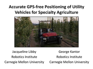
- 1. Accurate GPS-free Positioning of Utility Vehicles for Specialty Agriculture Jacqueline Libby Robotics Institute Carnegie Mellon University George Kantor Robotics Institute Carnegie Mellon University
- 2. USDA: CASC (Comprehensive Automation for Specialty Crops) Carnegie Mellon University Plant Science Automation Robotics Localization Outreach GIS Ag Economics
- 3. Why do we need positioning?
- 4. Why isn’t GPS enough? Cost Sub-meter accuracy prohibitively expensive Performance Line of sight to satellites occluded by trees New fruit wall structures Orientation complement GPS
- 5. Experimental Platform Drive-by-wire electric vehicle Brake and steering motors Internal sensors Wheel encoders External Sensors 2 Sick LMS 291 laser range scanners Ruggedized Dell laptop Receive data via Ethernet, USB Ground Truth Applanix POS 220 LV high-accuracy positioning system
- 7. Wheel Encoders Already used for vehicle control We use to measure relative motion
- 8. Laser Range Scanners Already used for safety, obstacle detection We use to measure range and bearing to landmarks
- 9. Map Known locations of landmarks Created offline with Applanix ground truth
- 10. Localization Filter Estimate vehicle pose Extended Kalman Filter Bayesian estimation technique
- 11. Let’s first look at the map…..
- 12. Creating the map
- 13. Creating the map
- 14. Wheel Encoders -> Prediction Step
- 15. Prediction Step: Dead Reckoning Given previous pose Steering and wheel encoder values Predict: current pose Assumptions: Bicycle model Error bad sensor data Wheel slip imperfect assumptions
- 16. Laser Range Scanners -> correction step
- 17. Correction Step
- 18. Correction Step
- 19. Correction Step
- 20. Correction Step
- 21. Correction Step
- 22. Correction Step
- 23. Extended Kalman Filter (EKF)
- 26. Tests and Results Error (m)
- 27. Conclusions and Future Work Very close to sub-meter accuracy goal Weakness: landmark spacing too dense Ongoing work: Improve prediction step: laser scan matching Improve measurement step: natural features Turning at the end of the row Future work Remove mapping step (SLAM) Other low-cost sensors (IMU, low-cost GPS)
Notas do Editor
- Here is a picture of the robotic vehicle we use in our work.You can see here that it is driving by itself, based on the navigation and control algorithms developed by our group.Goal: determine position and orientation of this vehicle to sub meter accuracy without GPSMotivation:Reliable and affordable technology for specialty agriculture.High accuracy GPS cost-prohibitive
- Pos info so fundamental to these types of systemsthat we often forget why it is significant.for example, allows data collected by on-board sensors to be geo-registered into maps this plot shows 3d point clouds from our laser range scanners other sensors, such as temperature and humidity, could be registered in a similar mannerAll this information can be collated into a GIS databaseThese photographs show examples of devices that could be towed on such a vehicle.This is a mower, and this is a weedseeker.This weedseeker both detects weeks and then sprays them.You could imagine that the information on where a week was detected, and where spraying occurred could be registered into a GIS data base. This could be used not only for record management, But for decision making purposes For example, a manager could decide on targeted areas for where further weedseeking should be performed. By targeting these areas, valuable chemicals and resources can be conservedOptional Automated vehicles Follow paths to targeted areas Safety Reduce human exposure to chemicals Reduce worker fatigue
- Line of sight to satellites is occluded by treesNot a problem in broad-acre crops, where GPS has been used successfully for many yearsEven in tall tree canopies, if tractors are tall enough, then signal interference not an issuebut for smaller utility vehicles, such as the one used in this work, vehicle must operate well below tree lineApple orchards, orange groves, almond groves: all examples of specialty agriculture where tall tree canopies would cause an issue for small vehiclesOther applications: environmental/biologicalForests, tree farmsi.e. monitoring carbon sequestrationNew fruit wall structures:Engineered to maximize light interception by the canopyRule out possibility of mounting antennas above the tree lineCost:GPS systems that provide sub-meter accuracy are prohibitively expensiveGPS gives position, but not orientation, of the vehicleAutomation: Needed for controlling turnsCollecting data: needed for determining the position of an object in the environment wrt the vehicleComplementary:In some applications, perhaps a cheap GPS can still be usedOut algorithms can complement this GPSProvide corrections when the GPS fails -> robustnessProvide orientation on top of positionMore accuracy
- Just talk about internal/external********************************drive-by-wire electric vehicleBrake and steering motors can be controlled by eitherHuman operatorAutonomous commands from an on-board computerInternal sensors: measure properties internal to vehicleEncoders: measure distance traveled and steering angleExternal sensors: measure properties of the environment2 Sick LMS 291 laser scannersSend out horizontal fan of beams, 180 degrees, 1 deg intervalsMeasure range and bearing to surrounding objectsRigidly attached, angled 30 degRuggedized Dell LaptopReceiving data via Ethernet and USBApplanix POS 220 LV high-accuracy positioning systemProvides ground truthPosition estimate: a few centimentersOrientation: 0.05 degrees
- Use sensors already on vehicle for other purposes:Wheel encoders provide measurements of vehicle motionAlready being used for controlWe use for prediction of relative position
- Laser range scannersAlready being used for safetyWe use to measure range and bearing to landmarks at known locationsCorrect our estimate of the vehicle’s pose
- Knowing the locations of the landmarks requires having a map We create the map offline with the help of ground truth form the applanixThis is done offline
- The main part of the algorithm is this feedback loop here.The wheel encoders provide a prediction of the vehicle’s position, which provides the dead reckoning step, in this boxThe lasers detect features in the map, which are used to correct this prediction which provides the correction step hereThe filter is then an iterative process that loops through this cycle as the vehicle moves through the world.
- List of (x,y) positions of landmarks in the environmentReflective tape, lasers read as high-reflectivity returnsDrive through the orchard, passing by landmarks multiple times from different anglesRecording data from both lasers and applanix1) We start with the a range and bearing measurement to a landmark2) With then re-write this as the x,y position wrt the laser frame3) The “H’s” shown in the diagram are what we call homogeneous transformation matricesAllow us to transform (x,y) coordinates from one frame to anotherLaser frame -> vehicle frameVehicle frame -> world frame4) Laser -> vehicle: fixed position and orientation – we calibrate for this5) vehicle -> world: applanixAs we drive up and down the orchard rows, we record the world coordinates of all the high-refl returns,As you can see here in this map with the pink dotsWe then use a clustering technique to take each local point cloud region and turn it into a single point feature for the mapShown by the x’s
- List of (x,y) positions of landmarks in the environmentReflective tape, lasers read as high-reflectivity returnsDrive through the orchard, passing by landmarks multiple times from different anglesRecording data from both lasers and applanix1) We start with the a range and bearing measurement to a landmark2) With then re-write this as the x,y position wrt the laser frame3) The “H’s” shown in the diagram are what we call homogeneous transformation matricesAllow us to transform (x,y) coordinates from one frame to anotherLaser frame -> vehicle frameVehicle frame -> world frame4) Laser -> vehicle: fixed position and orientation – we calibrate for this5) vehicle -> world: applanixAs we drive up and down the orchard rows, we record the world coordinates of all the high-refl returns,As you can see here in this map with the pink dotsWe then use a clustering technique to take each local point cloud region and turn it into a single point feature for the mapShown by the x’s
- given:Vehicle pose at time tSteering and wheel encoder values at time t+TFind:Vehicle pose at time t+TAssumption:Ackerman steeringDifferential drive 4-wheel vehicleSimplify to bicycle modelEuler approximation: curved -> point and shootEncoder on motor gives estimate of the forward velocityEncoder on the steering wheels gives us an estimate of direction the vehicle is traveling in -> angular velocity
- ReasonDead reckoning builds up error over timeUse measurements to landmarks to correct for this errorGiven:Actual measurement: range and bearing readings from laserModel of the measurement: Estimated vehicle (and laser) poseLandmark location, in mapLook at difference between actual measurement and measurement modelUse this to correct from our estimated laser pose closer to the actual laser pose
- ReasonDead reckoning builds up error over timeUse measurements to landmarks to correct for this errorGiven:Actual measurement: range and bearing readings from laserModel of the measurement: Estimated vehicle (and laser) poseLandmark location, in mapLook at difference between actual measurement and measurement modelUse this to correct from our estimated laser pose closer to the actual laser pose
- ReasonDead reckoning builds up error over timeUse measurements to landmarks to correct for this errorGiven:Actual measurement: range and bearing readings from laserModel of the measurement: Estimated vehicle (and laser) poseLandmark location, in mapLook at difference between actual measurement and measurement modelUse this to correct from our estimated laser pose closer to the actual laser pose
- ReasonDead reckoning builds up error over timeUse measurements to landmarks to correct for this errorGiven:Actual measurement: range and bearing readings from laserModel of the measurement: Estimated vehicle (and laser) poseLandmark location, in mapLook at difference between actual measurement and measurement modelUse this to correct from our estimated laser pose closer to the actual laser pose
- ReasonDead reckoning builds up error over timeUse measurements to landmarks to correct for this errorGiven:Actual measurement: range and bearing readings from laserModel of the measurement: Estimated vehicle (and laser) poseLandmark location, in mapLook at difference between actual measurement and measurement modelUse this to correct from our estimated laser pose closer to the actual laser pose
- ReasonDead reckoning builds up error over timeUse measurements to landmarks to correct for this errorGiven:Actual measurement: range and bearing readings from laserModel of the measurement: Estimated vehicle (and laser) poseLandmark location, in mapLook at difference between actual measurement and measurement modelUse this to correct from our estimated laser pose closer to the actual laser pose
- Iterative processPrediction and update steps coming in at different timesDependent on the frequencies of the various sensorsNot going into details here because not enough time….
- This localization algorithm was tested successfully in a variety of settingsSite description:The plot here shows results from experiments in apple orchard blocks at the Penn State Fruit Research and Extension CenterDuring the summer of 2009Total area of block: 60 square m6 50 m long rowsOrchard block was relatively new planting (~3yr old), trained in a vertical trellis systemExperimental SetupTraffic cones were placed throughout the orchardA total of 39 landmarks, shows as black dotsSpaced about 20 m apart in pairsFirst collect a data set to create the map, which was constructed offlineSubsequent experiments run to test the localization algorithm onlineGenerated real-time position estimates as the vehicle drove through the blockAfter the tests, results were analyzed to generate statistics on performancePlotResults of a typical runExplain colorsVeering slightly offWhen the vehicle goes for a fair amount of time without receiving measurements to landmarksWhen the measurement is finally received, the vehicle corrects itselfHistogramPrimary metric we use to quantify error is the euclidean distance between the estimate and ground truth at each timestepMean: 20cm, max: 1.2 mThe cumulative error distribution is plotted in red, with the scale on the rightThis shows us, for instance, that 90% of the time, the error is under 35 cm
- This localization algorithm was tested successfully in a variety of settingsSite description:The plot here shows results from experiments in apple orchard blocks at the Penn State Fruit Research and Extension CenterDuring the summer of 2009Total area of block: 60 square m6 50 m long rowsOrchard block was relatively new planting (~3yr old), trained in a vertical trellis systemExperimental SetupTraffic cones were placed throughout the orchardA total of 39 landmarks, shows as black dotsSpaced about 20 m apart in pairsFirst collect a data set to create the map, which was constructed offlineSubsequent experiments run to test the localization algorithm onlineGenerated real-time position estimates as the vehicle drove through the blockAfter the tests, results were analyzed to generate statistics on performancePlotResults of a typical runExplain colorsVeering slightly offWhen the vehicle goes for a fair amount of time without receiving measurements to landmarksWhen the measurement is finally received, the vehicle corrects itselfHistogramPrimary metric we use to quantify error is the euclidean distance between the estimate and ground truth at each timestepMean: 20cm, max: 1.2 mThe cumulative error distribution is plotted in red, with the scale on the rightThis shows us, for instance, that 90% of the time, the error is under 35 cm
- This localization algorithm was tested successfully in a variety of settingsSite description:The plot here shows results from experiments in apple orchard blocks at the Penn State Fruit Research and Extension CenterDuring the summer of 2009Total area of block: 60 square m6 50 m long rowsOrchard block was relatively new planting (~3yr old), trained in a vertical trellis systemExperimental SetupTraffic cones were placed throughout the orchardA total of 39 landmarks, shows as black dotsSpaced about 20 m apart in pairsFirst collect a data set to create the map, which was constructed offlineSubsequent experiments run to test the localization algorithm onlineGenerated real-time position estimates as the vehicle drove through the blockAfter the tests, results were analyzed to generate statistics on performancePlotResults of a typical runExplain colorsVeering slightly offWhen the vehicle goes for a fair amount of time without receiving measurements to landmarksWhen the measurement is finally received, the vehicle corrects itselfHistogramPrimary metric we use to quantify error is the euclidean distance between the estimate and ground truth at each timestepMean: 20cm, max: 1.2 mThe cumulative error distribution is plotted in red, with the scale on the rightThis shows us, for instance, that 90% of the time, the error is under 35 cm
- Scan to scan matching***********We have demonstrated sub-meter accuracy with current experimentsPrimary weakness: landmark spacing denser than is practicalWhen landmarks placed > 20m apart, dead reckoning becomes too largeAlgorithm will associate measurements to the wrong landmarkOngoing workImproving prediction stepLaser scan matching, more accurate dead reckoning, reducing driftImproving measurement stepNatural features:Entire tree rows: line featuresTree trunks: point featuresHard problem: turning at the end of rowWheel slipLaser odometry and better feature extractionFuture Work:SLAM (Simultaneous Localization and Mapping)No longer need expensive ground truthing for mapping stepOther low-cost sensors IMU’sPartial GPS EKF is a general sensor fusion techniquesLends itself to fusing data from multiple sensorsBy using multiple cheap sensors, we can provide affortable and reliable systems