SlideShare uma empresa Scribd logo
1 de 84
Baixar para ler offline
Investigating the distribution of small pelagic fish in Spanish
Mediterranean waters using environmental modelling,
essential fish habitat mapping and geostatistics
Alex Brown, 2006
Research project submitted in contribution to
MRes Marine and Fisheries Science
School of Biological Sciences (Zoology), University of Aberdeen, Scotland
I declare that this thesis has been composed by myself and has not been accepted in any
previous application for a degree. Information drawn from other sources and assistance
received has been duly acknowledged.
Signed:
21 August 2006
Alex Brown Date
Acknowledgements
I would like to acknowledge the provision of data and substantial contributions of time,
effort, advice and hospitality of my primary supervisor, José Ma
Bellido of the Centro
Oceanográfico de Murcia (IEO), whom it was always a pleasure to work with. Thank you
also to the many colleagues and friends who accomodated me in Murcia.
I am very grateful to Vasilis Valavanis of the Hellenic Centre for Marine Research
(HCMR) for providing data, accomodating me in Crete, and contributing many hours of
patient guidance towards the completion of this project. My gratitude extends to Andreas
Palialexis (HCMR) for his hospitality and technical advise.
I also thank Colin MacLeod of the University of Aberdeen who invested considerable
amounts of time and provided useful advice towards the completion of this project.
Finally, I am grateful to Paul Fernandes of Fisheries Research Services, Aberdeen, for
offering advice and providing me with the opportunity to participate in fieldwork related
to this project.
CONTENTS
1. INTRODUCTION 1
1.1 Environmental influences on the distribution of small pelagic fish
1.2 Essential Fish Habitat (EFH)
1.3 Geostatistics
1.4 Species ecology
1.5 Study area
1.6 Aims
2. METHODS 15
2.1 Survey data
2.2Allocation of zones
2.3 Environmental influences on the distribution of small pelagic fish
2.4 EFH mapping
2.5 Geostatistics
3. RESULTS 23
3.1 Environmental influences on the distribution of small pelagic fish
3.2 EFH mapping
3.3 Geostatistics
4. DISCUSSION 43
3.1 Environmental influences on the distribution of small pelagic fish
3.2 EFH mapping
3.3 Geostatistics
5. SUMMARY 51
REFERENCES 52
APPENDICES 57
Brown, 2006
1
1. INTRODUCTION
This study presents a multidisciplinary approach to investigating the distribution of small
pelagic fish. For clarity and ease of reading, the study is presented in three main themes:
environmental influences on the distribution of small pelagic fish, essential fish habitat
(EFH) mapping and geostatistics.
1.1 Environmental influences on the distribution of small pelagic fish
Small pelagic fish are predominantly confined to coastal regions, with the largest
populations occurring in regions of upwelling. The spatial heterogeneity of the physical
characteristics of the coastal pelagic environment, and the high mobility of small pelagic
fish, generally leads to their distribution within areas which they find most favourable
(Massé et al., 1996; Fréon et al., 2005). To a certain extent, fish show the ability to alter
their behaviour in order to adapt to such a variable environment (Agenbag et al., 2003).
However, all populations and species have an affinity for environmental conditions most
favourable to their survival, growth and reproduction (review in Blaxter & Hunter, 1982).
Fréon and Misund (1999) reviewed the environmental variables which have been related
to the distribution of small pelagic fish (hereafter referred to only as ‘fish’). Temperature,
salinity, dissolved oxygen, water transparency, light intensity, current, turbulence and
upwelling, depth in the water column, bottom depth and substrate have all been shown to
influence distribution at varying spatial and temporal scales. When studying
environmental influences at a regional scale, variables with high spatial coverage are
required. This places a major constraint on the environmental variables which can be
used in the analysis (Agenbag et al., 2003), hence the dominant use of remotely sensed
variables such as sea surface temperature (SST), sea surface chlorophyll-a concentration
(Chl-a) and bathymetry.
Using SST, an association between greater presence and abundance of fish and more
mixed waters and thermal fronts has been observed for a number of species, including
herring (Clupea harengus) in the northern North Sea (Maravelias & Reid, 1995);
Brown, 2006
2
anchovy (Engraulis ringens) and sardine (Sardinops sagax) off the coast of Chile
(Castillo et al., 1996); and sardine (Sardina pilchardus) and anchovy (Engraulis
encrasicolus) in the northern Aegean Sea (Giannoulaki et al., 2005). However, such
associations are commonly weak.
Relationships between abiotic environmental factors (e.g. temperature and salinity) and
fish distribution are likely to be indirect. In adult, non-spawning fish, the main factor
influencing their distribution is prey. The vast majority of adult fish are planktivorous,
and consume a combination of phytoplankton and zooplankton through filter or
particulate feeding (Longhurst, 1971 in Blaxter & Hunter, 1982). Abiotic factors may
provide an index for which biotic factors such as plankton abundance, which are more
directly related to fish distribution (Mendelssohn & Cury, 1987; Maravelias & Reid,
1995; Agenbag et al., 2003). Associations between high concentrations of plankton and
fish have been observed for C. harengus in the northern North Sea (Maravelias, 1999)
and anchovy (Engraulis mordax) in the eastern Pacific (Robinson, 2004).
At short time scales, environmental variability can change fish distributions with
considerable fishery implications (Fréon et al., 2005). Rapid horizontal and vertical
migrations can be induced, altering the distribution of fish and therefore their availability
to fishing. While many of these shifts in distribution may be relatively local and
temporary, they have been observed to persist for several months and over large areas,
greatly influencing the exploitation of populations (Schwartzlose et al., 1999; Binet et al.,
2001; Boyer et al., 2001; Bertrand et al., 2004).
Schwartzlose et al. (1999) described the fishery implications of expansion and contraction
of fish distribution. A larger area suitable for feeding and spawning may be beneficial to a
fish population in terms of recruitment potential. However, an expansion in distribution
will also alter their availability to fishing, possibly exposing them to more boats and
dangerously high levels of fishing mortality. Conversely, the dispersion of a population
over a greater area may reduce fishing mortality through increased difficulty in locating
shoals. Contraction of distribution to a smaller area may make the population more
Brown, 2006
3
available to those fleets which usually exploit them, and could be overexploited under
certain management regimes.
A wide range of methods for studying species distributions are now available including
generalised linear models (GLMs) and generalised additive models (GAMs) (review in
Guisan & Zimmermann, 2000). Both these techniques are frequently used to
simultaneously test the roles of several environmental factors on species distribution
(Guisan et al., 2002). GAMs use a link function to establish a relationship between the
mean of a response variable and a smoothed function of the explanatory variable(s), and
are able to deal with highly non-linear relationships, as are so often found in ecology
(Hastie & Tibshirani, 1986, 1990 in Guisan et al., 2002).
Many studies have used GAMs to study the distribution and abundance of marine species
in relation to environmental conditions, including several species of small pelagic fish
and cephalopods (e.g. Maravelias & Reid 1995; Bellido et al., 2001; Agenbag et al.,
2003). As described by Barry & Walsh (2002), problems associated with zero-inflated
data (as are commonly experienced with distribution data in ecology) can be avoided by
separately modelling presence/absence and abundance given presence of species with the
desired explanatory variables.
1.2 Essential Fish Habitat (EFH)
The identification of EFH can be regarded as an application of studying relationships
between fish distribution and the environment. The US Congress have defined EFH as
‘those waters and substrate necessary to fish for spawning, breeding, feeding, or growth
to maturity’, including the physical, chemical and biological properties of the marine
environment which support fish populations throughout their life cycle (DOC, 1997).
EFH therefore consists of an array of habitat distributions corresponding to each life
stage of a species. As described by Valavanis et al. (2004), habitat requirement
information is needed for each life history stage, including the range of habitat and
environmental variables with limiting effects on distribution.
Brown, 2006
4
In a study on the distribution of short-finned squid (Illex coindetti) in the eastern
Mediterranean Sea, Valavanis et al. (2004) used a Geographic Information System (GIS)
based methodology of EFH mapping. A development of this technique is currently being
applied to several sets of fishery data across the Mediterranean (including data used in
this study) in the EC project ‘Environmental Approach to Essential Fish Habitat
Designation’ (EnviEFH) (http://arch.imbc.gr/enviefh/). A combination of generalised
additive models (GAMs) and GIS tools are used to analyse environmental preferences of
species, then map EFH as areas of suitable environmental conditions. Where available,
existing life history information on species distribution are used as constraints.
The identification of EFH for commercial species may be used as a tool in spatial
components of fisheries management. For example, by identifying areas of EFH, fisheries
managers will be able to apply conservation measures to ensure the integrity of this EFH
is sustained. For less mobile fish, and particularly those with important benthic habitat
requirements, areas of EFH are likely to be fairly stationary over time. However, for
highly mobile fish such as small pelagic species, stationary benthic features are of limited
importance, particularly in non-spawning adults where feeding is the main activity (Fréon
& Misund, 1999).
As was described in section 1.1, environmental conditions such as temperature, salinity
and plankton abundance are frequently important habitat properties for small pelagic fish.
These conditions can show considerable spatio-temporal variability, therefore it is
essential to identify EFH at regular intervals in order to monitor variability in both the
quality and distribution of EFH.
1.3 Geostatistics
Geostatistics refers to a variety of techniques for analysing the spatial structure of a
resource. Initially developed for the exploitation of geological resources, geostatistics
have been used in the study of fish populations since the late 1980s (Rivoirard et al.,
Brown, 2006
5
2000). There are currently a wide range of techniques within the category of geostatistics,
which have many potential applications (Kaluzny et al., 1998). In fisheries science, these
techniques most frequently aim to quantify the level of spatial auto-correlation
(clustering) within a fish population in order to provide a more accurate estimate of total
abundance within a specified area (Maravelias et al., 1996; Maynou et al., 1998;
Rivoirard et al., 2000).
This study focuses on a combination of two complimentary tools which use sample data
to analyse the spatial structure of a fish population in order to create an estimation of total
abundance within a specified area. These are the variogram model and kriging, and are
described in detail by Kaluzny et al. (1998).
The variogram model
The spatial structure of a fish population can be described by an empirical variogram,
based on a variogram cloud. A variogram cloud is a scatterplot where each point is half
the mean-squared difference in value z (e.g. fish density) between pairs of sample points
separated by their geographic distance (h). The empirical variogram is a binned average
of the variogram cloud where h, termed the ‘lag’, represents a value of distance ± half
that distance (figure 1).
As standard, empirical variograms are omni-directional, in that they consider differences
between pairs of sample points in all directions. Before fitting a variogram model, several
uni-directional empirical variograms must be produced which each consider differences
only at certain orientations (e.g. 45°, 90°, 135°). If empirical variograms at different
orientations are clearly very different in structure, fish shoals are directional in shape, and
are said to be anisotropic. If anisotropy exists, it must be corrected for. If directional
empirical variograms are all similar, no corrections need to be made and a model can be
fitted to a standard omni-directional variogram.
Brown, 2006
6
A variogram model is produced by fitting a line of a specified shape through the points of
the empirical variogram. The line is fitted by minimising the residual sum of squares.
From the variogram model, the parameters: nugget, sill, range and objective are obtained
(figure 1). The nugget describes the amount of variance in z at very low distances. The
sill is where the variogram levels off, and describes the maximum amount of variance in
z. The range is the distance at which the sill is reached, and describes the distance at
which correlation vanishes. The range may be interpreted as the approximate diameter of
patches of fish. The objective is the residual sum of squares, and provides a measure of
the goodness of fit between the variogram model and empirical variogram.
Kriging
Kriging is an interpolation technique for point data which creates predictions of a value
(e.g. fish density) for a grid of specified points at a higher resolution than the sample
points (Kaluzny et al., 1998). Predictions are based on the values at sampling points and
the spatial structure of the fish population, as defined by the parameters nugget, sill and
range from the variogram model. Kriging allows better visualisation of fish distribution,
range
sill
nugget
Figure 1. Empirical variogram (points) with spherical model fitted (black line), showing the
parameters sill, nugget and range. X-axis = h (distance between sample points in nmi), y-axis
= gamma (half the mean-squared difference in fish density (log)). Objective = residual sum of
squares from spherical model.
Brown, 2006
7
and potentially more accurate estimates of abundance than are provided by sample points
alone.
1.4 Species ecology
A variety of species of small pelagic fish are present in Spanish Mediterranean waters.
They include sardine (Sardina pilchardus), anchovy (Engraulis encrasicolus),
Mediterranean horse mackerel (Trachurus mediterraneus), Atlantic horse mackerel
(Trachurus trachurus), round sardinella (Sardinella aurita), bogue (Boops boops), chub
mackerel (Scomber japonicus) and Atlantic mackerel (Scomber scombrus) (Giráldez,
2005). Although all of these species are caught by commercial fisheries, sardine and
anchovy have traditionally been the most commercially important (Pertierra & Lleonart,
1996), and have therefore been the main focus of scientific studies.
A common feature of the distribution of clupeoids such as sardine and anchovy is their
association with upwelling systems, productive bays and estuaries, or shallow, productive
continental shelves (Blaxter & Hunter, 1982). The productivity of these environments in
the western Mediterranean is initiated by hydrological processes such as river run-off,
upwelling of deep/slope waters to the surface, and mixing within the water column
(Estrada, 1996). These processes bring nutrient rich waters into the photic zone, allowing
phytoplankton growth. In the Mediterranean Sea, zooplankton abundance and distribution
are positively correlated with phytoplankton development (Champalbert, 1996).
Studies on the ecosystem functioning of the northwest Mediterranean have shown pelagic
species to dominate the total biomass, catches, and account for the greatest number of
flows between trophic levels (Tudela & Palomera, 1997; Coll et al., 2006). Sardine,
anchovy, and several other planktivorous small pelagic species play a major role in
western Mediterranean ecosystems by channelling energy from low to higher trophic
levels (Tudela & Palomera, 1997).
Brown, 2006
8
Both sardine and anchovy are planktivorous, usually feeding on a combination of
phytoplankton and zooplankton through filter-feeding and selective consumption of
larger prey (Blaxter & Hunter, 1982). A greater proportion of zooplankton is consumed
by anchovies than sardine (Louw et al., 1998), and studies on spawning aggregations of
anchovy in both the Gulf of Lions and Gulf of Valencia have shown a clear dominance of
copepod zooplankton in their diet (Tudela & Palomera, 1997; Plounevez & Champalbert,
2000).
In the western Mediterranean, anchovy spawn and are mainly caught in spring and
summer when the majority of individuals are 1 year old (Palomera, 1992; Pertierra &
Lleonart, 1996). Sardine spawning extends from October to May, with a peak during
winter (Olivar et al., 2001), while they are caught mostly in the spring and autumn when
the majority of individuals are between 1 and 2 years old (Lloret et al., 2004).
Temperature preferences for spawning are between 15-22°C for anchovy (García &
Palomera, 1996) and below 20°C, with increased intensity below 18°C, for sardine
(Olivar et al., 2003). The temperature preferences of adult anchovy and sardine in the
western Mediterranean are undocumented outside of spawning events. However, in the
northern Aegean Sea Giannoulaki et al. (2005) showed non-spawning sardine to occupy
warmer waters than spawning anchovy, with the suggestion that warmer waters provided
favourable conditions for somatic growth.
1.5 Study Area
The study area comprises the entire Mediterranean coast of Spain. This extends from the
southern Gulf of Lions in the north, through the Gulf of Valencia to the south, before
ending at the Strait of Gibraltar in the western Alboran Sea (figure 2). A study area
boundary is defined to encompass the continental shelf (to 200m depth contour)
environment (coastline to 200m depth contour) and a small area immediately offshore of
this.
Brown, 2006
9
The Mediterranean Sea is generally considered an area of low, but fairly stable
productivity (Margalef, 1985). However, many areas of higher productivity exist where
oceanographic and meteorological conditions are favourable for primary productivity
(Lloret et al., 2004). Several such features have been identified in the Spanish
Mediterranean.
The Gulf of Lions and Gulf of Valencia
In the north, the Gulf of Lions is a well documented region of high productivity, caused
by a combination of a fairly wide continental shelf; considerable river run-off from the
Rhône; and a high degree of wind-induced mixing and upwelling from the strong,
predominantly north-westerly winds blowing in this region (Estrada, 1996; Salat, 1996;
Figure 2. The study area and its surrounding geography. Including nearby cities
and major rivers draining into the study area.
Brown, 2006
10
Agostini & Bakun, 2002). Slightly to the south, fertilization of Catalan shelf waters is
caused by local vertical mixing and intrusions of slope waters onto the shelf through
submarine canyons (Salat et al., 2002). The influence of these processes in the Gulf of
Lions and Catalan shelf extend south along the Spanish coast through the passage of the
Northern Current. Also known as the Liguro-Provencal-Catalan Current, the Northern
Current flows in a south west direction along the continental slope from the Gulf of
Genoa to the Gulf of Valencia (figure 3) (Millot, 1987 in Millot, 1999; Font et al., 1995).
Fresh, nutrient enriched waters from the rivers Rhône and Ebro become entrained in the
Northern Current, producing a shelf/slope haline front between the less saline coastal
waters and more saline offshore water (Font et al., 1995). The Northern Current exhibits
increased strength and mesoscale activity during winter months due to greater wind
forcing (Millot, 1999). In the Gulf of Valencia, the wide Iberian shelf deflects the
Northern Current further offshore. Here, coastal waters are more influenced by local
Figure 2. The path of the Northern Current along the continental slope of the
north-western Mediterranean. Source: Font et al. (1995).
Brown, 2006
11
meteorological events and freshwater inputs (Salat, 1996). Salat et al. (2002) suggested
that nutrient inputs from the Ebro outflow may account for 10-25% of the total nutrient
content in the waters of the adjacent Iberian shelf. In addition to riverine inputs in this
area, nutrient enrichment also occurs around the Ebro delta as a result of intense water
mixing on the wide shelf, induced by the strong north-westerly winds associated with this
region (Estrada, 1996; Salat, 1996).
Regional enrichment events such as those described above have been shown to greatly
influence the productivity and fishing activity associated with anchovy on the Iberian
shelf (Palomera, 1992; Agostini & Bakun, 2002; Lloret et al., 2004). The Gulf of Lions
and Iberian shelf around the Ebro delta are the main spawning areas of anchovy in the
northwest Mediterranean (García & Palomera, 1996). They also provide important
sardine spawning habitats (Olivar et al., 2001). The prevalence of sardine and anchovy in
these waters is confirmed by a high level of fishing activity, where pelagic trawl and
purse seine techniques yield some of the highest landings of these species in the
Mediterranean (Pertierra & Lleonart, 1996).
The Alboran Sea
In addition to the Gulfs of Lions and Valencia, the Alboran Sea is another well
documented area of productivity within the western Mediterranean. Agostini & Bakun
(2002) identified the Alboran Sea, along with the Gulf of Lions and adjacent Catalan
coast, as two of five ‘ocean triad’ regions in the Mediterranean. Ocean triads are defined
as areas of high productivity, with enrichment, concentration and retention processes
favourable for reproduction and growth in coastal pelagic fishes (Bakun, 1998).
Wind-driven processes of nutrient enrichment are less intense in the Alboran than the
north-west Mediterranean (Agostini & Bakun, 2002), the continental shelf is very narrow,
and there are no major river inputs. Instead, the input of cooler, less saline, nutrient rich
Atlantic surface water at the Strait of Gibraltar dominates the hydrographic
characteristics of the region. A ‘jet’ of Atlantic water causes turbulent mixing in the
Brown, 2006
12
Strait, and the development of two anticyclonic gyres in the Alboran Sea (figure 4) with
associated upwelling on the Spanish coast (Tintorè et al., 1991; Estrada, 1996). All of
these processes cause areas of enhanced primary productivity and corresponding high
zooplankton concentrations along the Spanish Alboran coast (Estrada, 1996;
Champalbert, 1996; Viudez et al., 1998).
Along with the Gulf of Lions and Iberian shelf, the Alboran Sea represents an important
area of anchovy concentration and fishing in the western Mediterranean (Garcia &
Palomera, 1996). The Bay of Málaga has been identified as an anchovy and sardine
nursery ground, and the transport of eggs and larvae into the Mediterranean from
spawning grounds in the Atlantic has been shown (García & Palomera, 1996).
Costa Blanca and Golf of Vera
There is little mention in the scientific literature of the oceanographic processes taking
place in the Costa Blanca and Gulf of Vera. These regions form something of a transition
zone between the influence of the Northern Current in the north, and the Algerian current
in the Alboran Sea (Millot, 1999). The continental shelf is very narrow in the Gulf of
Vera and there are no major freshwater inputs into the area. The latter is also true of the
Costa Blanca, as discharge from the River Segura is minimal (Bellido, pers. comm.).
However, the continental shelf is fairly wide, and it is likely that this region is somewhat
Figure 4. Circulation in the Alboran Sea, showing Western and
Eastern Alboran Gyres (WAG and EAG respectively), and the
associated Algerian Current. Source: Baldacci et al. (2001).
Brown, 2006
13
influenced by processes further north (Millot, 1987 in Millot, 1999). Anchovy catches are
traditionally low in the Gulf of Vera region (García & Palomera, 1996).
1.6. Aims
This study aimed to use a GIS-based environmental modelling approach to investigate
relationships between the distribution and abundance of small pelagic fish and
environmental conditions in Spanish Mediterranean waters. A further aim was to apply
an extension of this approach to sardine and anchovy specifically, in order to identify
EFH and its temporal variability. Finally, geostatistics were to be used to further
investigate the distribution and abundance of fish.
These aims were achieved by undertaking the following specific tasks:
Environmental influences on the distribution of small pelagic fish
1. Develop a GIS for the purpose of storing, integrating, processing and visualising
survey and environmental data.
2. Model relationships between the presence/absence of fish and environmental
conditions for each zone and year, using only the presence/absence of fish.
3. Model relationships between abundance of fish and environmental conditions for each
zone and year, using data only where fish are present.
EFH mapping
4. Repeat task 2 but using the presence/absence of sardine and anchovy, rather than small
pelagic fish in general, and only for all years combined.
5. Select models produced in task 4, and use these to predict the probability of presence
of sardine and anchovy throughout the study area in each year.
Brown, 2006
14
6. Using predictions from task 5, produce maps to visualise the spatial distribution of
EFH.
7. Analyse spatial and temporal trends in the distribution and quality of EFH between
years.
Geostatistics
8. Process acoustic data to obtain values of fish density per nmi2
for use in geostatistical
analyses.
9. Using values of fish density obtained in task 8, produce variogram models to analyse
the spatial structure of sardine and anchovy distributions in each zone and year.
10. Based on the variogram models produced in task 9, perform kriging to interpolate
values of fish density to a higher resolution than that of the survey data. Then, use kriged
values to estimate the total abundance of fish throughout the study area.
Brown, 2006
15
2. METHODS
2.1 Survey Data
Biological data were collected by the Instituto Español de Oceanografía (IEO) aboard the
Research Vessel Cornide de Saavedra during annual acoustic surveys. The surveys began
in the north at the France/Spain border (42.42°N, 3.43°E) in the penultimate week of
November, before progressing south and east to finish at the Strait of Gibraltar (36.13°N,
5.26°W) approximately 4 weeks later. The entire Spanish Mediterranean coast is
surveyed in a total of 128 individual transects covering a distance of 1270 nautical miles
(nmi). Transects are oriented perpendicular to the coast and parallel to each other, with
the intention of surveying the continental shelf between the 30m and 200m isobaths
(figure 4). Transect length was a minimum of 5 nmi, so the survey extended slightly
beyond the 200m isobath in areas of extremely narrow continental shelf. Transects were
separated by 4 nmi in areas where the continental shelf is narrow (zones 1 and 3), and 8
nmi where the shelf is wide (zone 2).
Acoustic equipment comprises a SIMRAD EK-500 scientific echosounder operating at
38 KHz with a split beam transducer, and an additional SIMRAD EY-500 echosounder.
The echosounders were calibrated prior to commencing each survey in accordance with
the standard 60mm copper sphere method (Foote et al., 1987). Acoustic signals were
integrated into Elementary Distance Sampling Units (EDSUs) for every 1 nmi surveyed.
Acoustic signals were later processed using Sonar Data’s Echoview software to remove
signals not attributable to fish, and give a total Nautical Area Scattering Coefficient
(NASC) value per EDSU. NASC describes m2
of cumulative backscattering cross section
per nmi2
, and is considered a measure of abundance in this study. A species composition
was assigned to each NASC based upon experimental fishing in the vicinity of the EDSU
(as described in MacLennan and Simmonds, 1992). Acoustic surveying took place
between the hours of 06:00 and 18:00, with experimental fishing at night.
The surveys described above generated 1290, 1292 and 1268 records for 2003, 2004 and
2005 respectively with almost exact spatial overlap between years. Each record describes
Brown, 2006
16
the central longitude and latitude, NASC and species composition of each EDSU. For the
years 2004 and 2005, data were also available describing the mean length frequency
distribution of each species for the total survey area (obtained through experimental
fishing). This allowed the calculation of fish density from NASC for these two years.
2.2 Allocation of zones
The study area was divided into 3 zones, which were considered throughout all analyses
(figure 5). As described in section 1.5, oceanographic and fishery characteristics vary
considerably throughout the study area, and therefore it is sensible to consider fish –
environment relationships at different spatial scales.
For geostatistical purposes, the boundaries of zones are defined according to inter-
transect distance used in the survey. Zones 1 and 3 are areas of fairly narrow continental
shelf where transects are separated by 5 nmi, in contrast to the 8 nmi spacing in zone 2.
Consistent inter-transect spacing is advisable when considering the spatial structure of
fish assemblages (Rivoirard et al., 2000)
Figure 5. Map showing the extent of zones 1 (blue),
2 (red) and 3 (green), and transects locations (black
lines).
Brown, 2006
17
In addition to geostatistical considerations, differences in the geography and
oceanography of the Spanish Mediterranean coast are well represented by these zones.
Zone 1 faces predominantly east and south east, and is influenced by the Northern
Current and processes taking place in the Gulf of Lions. Zone 2 faces predominantly
south east, and is dominated by the wide Iberian shelf and its associated hydrological
features. Zone 3 is an area of extremely narrow continental shelf, with the south facing
Alboran coast influenced by inflow of Atlantic waters, and the south east facing Gulf of
Vera representing a transition zone between southern and northern hydrographic
processes.
2.3 Environmental influences on the distribution of small pelagic fish
GIS development and environmental data
A GIS was developed using Environmental Systems Research Institute’s ARC/INFO and
ArcView 3.3 software. A large number of environmental data were collated from
internet-based sources by the Hellenic Centre for Marine Research1
, then processed into
files suitable for use in a GIS (table 1). These data overlapped temporally with the dates
of surveys (November and December 2003, 2004 and 2005). The spatial resolution of
these data varied from one source to another, so all were converted to the same resolution
as sea surface temperature (which had the highest resolution) using the ‘Topogrid’
interpolation function in ARC/INFO. Point covers of fisheries records were combined
with environmental grids to extract environmental values for each fisheries record. Care
was taken to ensure the temporal resolution of the environmental grid matched that of the
fisheries sampling date. Maps were produced to visualise the distribution of NASC
values throughout the study area.
1
Hellenic Centre for Marine Research, Crete, Greece. www.hcmr.gr
Brown, 2006
18
Variable Units Source Sensor/Model URL
Photosynthetically Active
Radiation (PAR)
(E/m2
/d) Oceancolor WEB,
GSFC/NASA, USA
SeaWiFS http://oceancolor.gsfc.nasa.gov
Sea Level Anomaly
(ALT)
cm Live Access Server, Merged (TOPEX/Poseidon, Jason-1,
ERS-1/2, Envisat)
http://www.aviso.oceanobs.com/
Sea Surface Temperature
(SST)
°C DLR EOWEB, Germany AVHRR SST http://eoweb.dlr.de:8080/
Sea Surface Chlorophyll-a
Concentration (Chl-a)
(mg/m3
) Oceancolor WEB,
GSFC/NASA, USA
SeaWiFS http://oceancolor.gsfc.nasa.gov
Sea Surface Salinity
(SSS)
psu IRI/LDEO, USA CARTON-GIESE SODA and CMA
BCC GODAS
http://ingrid.ldeo.columbia.edu/
Wind Speed (WS) (m/sec) RS Systems, USA QuikSCAT http://www.ssmi.com/
Wind Direction (WD) (° from N) RS Systems, USA QuikSCAT http://www.ssmi.com/
Bathymetry (depth) m NGDC, NOAA, USA Geostat ERS-1 satellite & ship depth
echosoundings
http://www.ngdc.noaa.gov/mgg/
image/2minrelief.html
Table 1. Sources and descriptions of environmental data used in the GIS
Brown, 2006
19
Generalised Additive Models (GAMs)
Despite having a choice of 8 different environmental variables to use as explanatory
variables in GAMs (hereafter referred to as ‘models’), it was decided that many were
unsuitable for this type of model. For example, there was collinearity amongst several of
the variables, and some showed very little variability throughout the study area (eg. SSS,
WS, WD). SST, Chl-a and depth were selected for models as they showed considerable
variability and were believed to be easier to interpret biologically than some other
variables available.
To overcome problems associated with the zero-inflated nature of our data, a two-stage
modelling process was used as suggested in Barry & Welsh (2002). Firstly, only the
association between presence/absence of fish and the environmental variables was
modelled. In the second step, only records with species presence were used so that the
association between NASC and environmental variables could be modelled.
Modelling procedure
Highland Statistic Ltd’s ‘Brodgar’ interface for ‘R’ was used to carry out the modelling.
Models were produced for both the entire survey area, and for each of the three zones
described in section 3.2. This was done for each year individually, in addition all years
combined.
For presence/absence models, a binomial or quasibinomial (where the overdispersion
parameter exceeded 1.0) distribution and logit link function were used. In models using
NASC as a response variable, a poisson distribution and log link function were used. All
environmental variables were used as smoothing terms. Due the presence of several
extreme values, a natural log transformation was applied to SST, Chl-a, depth and NASC.
Brown, 2006
20
For each model, a forward step-wise selection method was used to select the combination
of environmental variables which produced the best model in terms of the lowest possible
AIC. The deviance explained and significance of each variable was noted, but did not
influence the choice of model. Where collinearity existed between variables, they were
modelled separately before selecting the variable which produced the best model. Cross
validation was applied during modelling to estimate the optimum number of degrees of
freedom of each smoother. Classification trees (for presence/absence) and regression
trees (for NASC) were produced for each combination of variables in the best models.
This allowed the relative importance of each variable in a model to be calculated. The
detailed properties of trees were not considered in the analyses.
2.4 EFH mapping
As sardine and anchovy have traditionally been the most economically important species
in the Spanish Mediterranean (Pertierra & Lleonart, 1996), they were both chosen for
EFH mapping. The GAM procedure described in section 2.3:’modelling procedure’ was
repeated using presence/absence data for sardine and anchovy, although models were
only produced using all years combined – not individual years.
Through the GIS, boundaries were defined to encompass the surveyed points and the
surrounding area. Within each boundary, point values were extracted from each of the
environmental data grids and merged into spreadsheet files, providing high resolution
data of the environmental conditions in each year. Using the statistical package R,
presence/absence models were used to predict the probability of species presence for the
aforementioned high resolution environmental data. The predictions were then mapped as
grids.
Once the probability of species presence was predicted for the entire area, both species
and each year, the characteristics of these predictions were analysed. Scatterplots
comparing predictions between years provided qualitative visual analysis of inter-annual
differences in predictions at specific locations. Cumulative frequency plots enabled the
Brown, 2006
21
comparison of predictions for an entire area. Kolmogorov-Smirnov (KS) tests were used
to statistically quantify differences in the frequency distribution of predictions between
years.
2.5 Geostatistics
Data processing
Spreadsheets were developed to convert the NASC of each record into fish density for
each species, as no existing conversion tools were designed to deal with either this
volume of data or number of species. As with EFH mapping, only sardine and anchovy
were selected for geostatistical analysis. However, it was essential to calculate fish
density of all species in order to accurately apportion the NASC between species.
A target strength of 20log(L) -71.9 (where L is the fish length (cm) and -71.9 is a
constant) was used for all species. Target strengths estimates have been shown to vary
between different species of similar fish, between different areas, and according to the
size range of fish considered (review in Simmonds & MacLennan, 2005). However, in
the absence of calculated target strengths for any of the species surveyed in this area, the
value of 20log(L) -71.9 seemed most appropriate as it is based on calculations from a
variety of clupeoid fishes of many length classes in a variety of areas (Foote, 1987 in
Simmonds & MacLennan, 2005). It was decided that, based on target strength
information available, this value would be the least likely to cause large errors in
abundance estimates of any one species.
The variogram model
All geostatistical analysis was performed using Insightful’s S-PLUS software package
with Spatial Stats module, following the methods described in Kaluzny et al. (1998).
Variograms used fish density data, and were produced for each species, zone and year.
Units of longitude and latitude were converted from decimal degrees to x and y co-
Brown, 2006
22
ordinates in nmi. For empirical variograms, the lag was specified as 1 nmi greater than
the inter-transect distance for zones 1 and 3, and 2 nmi greater than the inter-transect
distance for zone 2. This allowed the variograms to consider differences in fish density
between neighbouring transects. Multi-directional empirical variograms confirmed an
absence of anisotropy for all species, zones and years.
Omni-directional empirical variograms were fitted with spherical models (appendices 19
– 20). The fit was optimized through minimizing the residual sum of squares. The
variogram model provided the parameters nugget, sill and range for each species, zone
and year.
Kriging
Polygons were manually defined for each zone to encompass the surveyed points. New
sampling grids with a resolution of 1 nmi2
were defined within each polygon. Using the
parameters obtained from variogram models described above, ordinary kriging was
performed on the surveyed fish density values. This produced predicted values of fish
density for the new sampling grid which could be mapped in the GIS. As the units of fish
density were fish nmi-2
, and the resolution of kriged predictions was 1 nmi2
, the sum of
fish density data per zone provided estimates of total abundance.
Brown, 2006
23
3. RESULTS
3.1 Environmental influences on the distribution of small pelagic fish
Visualising the distribution of NASC
The mapping of NASC values for each zone and year allowed visualization of spatial and
temporal trends in the distribution of fish (figures 6-8). The addition of a layer displaying
Chl-a allowed the distribution of fish to be visualised relative to this environmental
variable.
In zone 1, there are two main areas where the greatest NASC values were found (figure
6). One of these areas existed at the northern limits of the survey, in the southern Gulf of
Lions where the coast faces east. This area also showed some of the highest Chl-a in the
zone. NASC values in this area were highest in 2003. Another zone of consistently high
NASC existed north and south of Barcelona, also where higher Chl-a was seen. Again,
2003 showed the highest values of NASC.
In zone 2, high NASC values were most abundant in the north, where the continental
shelf is wide and Chl-a was generally high (figure 7). A peak in Chl-a existed around the
delta of the River Ebro, but high NASC values were not restricted to this area. South of
the Gulf of Valencia, along the Costa Blanca, several locations showed a high NASC,
although these were patchier in distribution than in the north. NASC values were
noticeably lower in 2004 compared to other years.
In zone 3, high NASC values were seen almost all along the narrow continental shelf
(figure 8). These were most consistent in the western Alboran Sea, which was also an
area of high Chl-a. In 2005, notably higher Chl-a was seen in the Gulf of Vera.
Interestingly, a small area of very high Chl-a showed a complete absence of fish. NASC
values were generally lower in 2004 compared to other years
Brown, 2006
24
2003
2004
2005
Figure 6. Zone 1 NASC and Chl-a
for 2003 – 2005.
Brown, 2006
25
2004
2003
2005
Figure 7. Zone 2 NASC and Chl-a
for 2003 – 2005.
Brown, 2006
26
Figure 8. Zone 3
NASC and Chl-a for
2003 – 2005.
2003
2004
2005
Brown, 2006
27
Presence/Absence Data
The proportion of records with fish presence showed considerable spatial and temporal
variation (table 2). 2005 yielded the highest proportions of fish presence, 2004 the lowest,
with 2003 slightly higher than 2004. Generally, zone 1 showed the highest proportions of
fish presence, with zone 2 slightly lower, and zone 3 the lowest. There were some
exceptions to this trend, particularly zone 1, 2003, which exhibited a lower proportion of
presence than the general trend suggests.
Year Zone Records with fish
present/absent
Proportion
with fish present
2003 All
1
2
3
658 / 632
137 / 155
360 / 301
161 / 337
0.510
0.469
0.545
0.478
2004 All
1
2
3
603 / 689
152 / 149
310 / 352
141 / 188
0.467
0.505
0.468
0.429
2005 All
1
2
3
778 / 490
201 / 99
414 / 236
163 / 155
0.614
0.670
0.637
0.513
All All
1
2
3
2039 / 1810
490 / 403
1084 / 889
465 / 518
0.530
0.549
0.549
0.473
GAMs were able to explain between 21.3% and 51.5% of the deviance in fish
presence/absence (table 3). Some common trends in these results were apparent. Models
for zone 1 explained the least deviance, followed by models for all zones combined.
Generally, the greatest proportion of deviance was explained by models for zone 3.
However, in 2005, the model for zone 2 explained the most deviance. When considering
all zones combined, the greatest proportion of deviance was explained by the model for
2005, followed by 2003, then all years combined, and then 2004.
Table 2. Presence/absence of fish records for each
zone and year, including the proportion of records
with fish present
Brown, 2006
28
In all models, depth was the most important variable and was always highly significant.
The relationship between depth and fish presence/absence was generally strongly
negative with increasing depth, although a few models did show fluctuations in this trend
at more shallow depths (appendices 1 - 4). For the majority of models, depths in excess of
approximately 100m (4.6 on natural log scale) had a negative effect on fish presence.
Another common characteristic was a small peak in the positive influence of depth on
fish presence between approximately 35 – 60m (3.5 – 4.1 on natural log scale) (figure 9).
Chl-a was frequently the second most important variable, and was significant in all
models except zones 1 and 2 in 2004. The relationship between fish presence/absence and
Chl-a was fairly weak and positive, with increasing chlorophyll-a concentration generally
leading to greater fish presence. At very high Chl-a, the relationship was subject to
considerable uncertainty due to a low number of values (figure 9).
SST was the least frequently used variable, although it was still included in 11 of the 16
models produced. It was generally the least important variable, and was often non-
significant. However, it was more important than Chl-a in 3 out of 4 models for zone 3.
Whenever co-linearity existed between Chl-a and SST, chlorophyll was always the more
important of the two variables. The character of the relationship between SST and fish
presence/absence varied spatially and temporally, and was generally very weak. In zone
3, there was a negative relationship between increasing SST and fish presence. In other
zones, the relationship often showed a peak in positive influence on fish presence
between approximately 16°C and 17°C (2.77 – 2.83 on natural log scale) (figure 9).
Brown, 2006
29
Year Zone n Variables (p-value) Deviance Explained (%)
2003 All
1
2
3
1290
292
661
337
depth (<0.01), Chl-a (<0.01), SST (0.23)
depth (<0.01), Chl-a (<0.01),
depth (<0.01), Chl-a (<0.01), SST (0.40)
depth (<0.01), SST (<0.01)
32.6
21.3
35.7
50.1
2004 All
1
2
3
1292
301
662
329
depth (<0.01), Chl-a (<0.01)
depth (<0.01), Chl-a (0.08), SST (<0.01)
depth (<0.01), Chl-a (0.07)
depth (<0.01), Chl-a (<0.01)
29.3
26.5
30.6
44.1
2005 All
1
2
3
1268
300
650
318
depth (<0.01), SST (<0.01)
depth (<0.01), Chl-a (<0.05)
depth (<0.01), Chl-a (<0.05), SST (<0.01)
depth (<0.01), SST (0.78), Chl-a (<0.05)
39.7
33.4
51.5
48.7
All All
1
2
3
3849
893
1973
983
depth (<0.01), Chl-a (<0.01), SST (<0.01)
depth (<0.01), SST (<0.01), Chl-a (<0.01)
32.3
24.5
36.3
45.3
Table 3. Fish presence/absence GAM results, showing the best model for each zone
and year. Variables are ordered according to their importance in the model, based on
results from classification trees. The order runs from left (most important) to right
(least important). Non-significant variables are highlighted in red.
Brown, 2006
30
Figure 9. Fish presence/absence GAM plots, all years combined. X-axis = explanatory
variable used as a smoother (natural log scale), depth (left), Chl-a (middle), SST (right). Y-axis
= influence of smoother on the presence of fish. Dashed lines represent 95% confidence
interval.
Fish presence/absence GAM plots, all years combined
Zone 3
Zone 2
Zone 1
All zones combined
Brown, 2006
31
NASC Data
GAMs were able to explain between 2.03% and 16.2% of the deviance in NASC (table
4). When considering all zones combined, the greatest proportion of deviance was
explained by the model for 2005, followed by 2003, then all years combined, then 2004.
This was the same trend as was seen using presence/absence data. However, when
considering individual zones, models for zones 1 and 2 in 2005 explained the least
deviance of all years, whereas zone 3, 2005 explained the most.
The choice of variables used in models varied considerably both spatially and temporally,
with no obvious consistent trends between years or zones. Depth was the most frequently
used variable, included in 13 of the 16 models, followed by SST (8 out of 16 models),
then Chl-a (6 out of 16 models). Chl-a was not used in any models for 2005, and SST was
only used in 2005 for all zones combined.
Where depth was used, it showed a negative relationship with NASC, similar to that
between depth and fish presence/absence, although the relationship with NASC more
weak. The influence of depth on fish presence became negative at depths in excess of
approximately 60m (4.1 on natural log scale) (figure 10, and appendices 5 - 8).
The relationship between Chl-a and NASC was similarly positive to that of chlorophyll
and fish presence/absence, with increasing Chl-a showing an increasingly positive effect
on NASC (figure 10, and appendices 5 - 8). As with presence/absence models, this
relationship was generally weak, and there was considerable uncertainty in this
relationship at very high Chl-a due to a low number of values.
The character of the relationship between SST and NASC varied spatially and
temporally, and was often weak. In all zones combined and zone 3, there was a negative
relationship between increasing SST and NASC. For zone 1, there was a weak positive
relationship between SST and NASC, although this was non-significant in all years.
Brown, 2006
32
Year Zone n Variables (p-value) Deviance Explained (%)
2003 All
1
2
3
658
137
360
161
Chl-a (<0.01), depth (0.09), SST (<0.05)
Chl-a (<0.01), SST (0.15)
SST (<0.01) , depth (0.46)
depth (0.07)
11.3
12.6
14.1
2.81
2004 All
1
2
3
603
152
310
141
depth (<0.05), Chl-a (<0.05)
depth (<0.01), SST (0.56)
Chl-a (<0.01)
SST (0.26)
6.13
14.1
5.65
2.83
2005 All
1
2
3
778
201
414
163
SST (<0.01), depth (0.20)
depth (0.35)
depth (<0.01)
depth (<0.01)
16.2
2.03
4.16
5.43
All All
1
2
3
2039
490
1084
465
Chl-a (<0.01), depth (<0.01), SST (0.12)
depth (<0.01)
depth (<0.01), Chl-a (<0.05), SST (0.15)
SST (<0.01), depth (0.15)
7.65
4.89
7.46
10.3
Table 4. NASC GAM results, showing the best model for each zone and year. Variables
are ordered according to their importance in the model, based on results from regression
trees. The order runs from left (most important) to right (least important). Non-
significant variables are highlighted in red.
Brown, 2006
33
Figure 10. NASC GAM plots, all years combined. X-axis = explanatory variable used as a
smoother (natural log scale), depth (left), Chl-a (middle), SST (right). Y-axis = influence of
smoother on the NASC. Dashed lines represent 95% confidence interval.
NASC GAM plots, all years combined
Zone 3
Zone 2
Zone 1
All zones combined
Variable not
used
Variable not
used
Variable not
used
Brown, 2006
34
3.2 EFH Mapping
GAMs revealed relationships between the presence/absence of sardine and anchovy and
environmental conditions (appendices 9 - 11). The characteristics of these relationships
are not discussed in detail here, but they can be described as generally similar to those
identified in section 3.1:’presence/absence data’ between fish presence/absence and
environmental conditions.
For sardine, models explained 23.9%, 36.3% and 40.3 % of the deviance for zones 1, 2
and 3 respectively (appendix 9). For anchovy, models explained 26.5%, 37.2% and 33.6
% of the deviance for zones 1, 2 and 3 respectively (appendix 9). All models used depth,
SST and Chl-a, except anchovy, zone 3, which did not use SST.
Mapping of the predictions allows visual analysis of the distribution and quality of fish
habitat (figure 11, and appendices 12 - 13). In this study, EFH is not defined as habitat
with a predicted probability of presence above a specific threshold value. Instead, all
areas within the study area are referred to as EFH, with comparisons being made in
accordance with the quality of this EFH. Higher predictions clearly indicate better quality
habitat, in terms of the environmental variables considered in the model on which the
predictions are based.
Zone 1 showed the greatest inter-annual variation in the quality of EFH (figure 11). For
both species, areas of high predictions were similar to those of higher NASC values as
described in section 3.1: ‘visualising the distribution of NASC’. These included the
southern Gulf of Lions and areas north and south of Barcelona. 2005 clearly showed the
highest predictions, which were also the most widespread high predictions of all the
years. 2003 showed fairly high predictions in the southern Gulf of Lions and south of
Barcelona, but low predictions north of Barcelona. In 2004, the habitat appeared to be of
good quality around Barcelona, but there were very low predictions in the southern Gulf
of Lions. This was most apparent for anchovy, where a probability of presence was rarely
predicted above 0.3 in this area.
Brown, 2006
35
Sardine, 2003 Sardine, 2004 Sardine, 2005
Anchovy, 2003 Anchovy, 2004 Anchovy, 2005
Figure 11. EFH maps
showing the predicted
probability of presence
of sardine and anchovy
in zone 1 for 2003,
2004 and 2005.
Brown, 2006
36
Inter-annual trends in the quality of EFH were further analysed through cumulative
frequency plots (figure 12) and scatterplots (figure 13). KS tests quantified inter-annual
differences in the frequency distributions of EFH predictions (table 5). Cumulative
frequency plots showed zone 1 to exhibit the greatest inter-annual differences in EFH
(figure 12, and appendix 15). In this zone, the same trend in differences was apparent for
both sardine and anchovy, although differences were of a greater magnitude for anchovy.
While the quality of EFH in years 2003 and 2004 appeared similar, 2005 was quite
different. A cumulative frequency of 1 was reached at a much higher predicted
probability of presence in 2005. This indicated a greater proportion of higher predictions
in 2005, particularly for predictions in excess of approximately 0.7 – where the graph
steepened.
KS tests calculated the maximum difference between the cumulative frequencies of
predictions in each year (KS-value), and the significance of these differences (table 5).
KS-values were greater for anchovy than sardine in all zones and between all years (with
the exception of zone 2, 2004 vs 2005, where values were the same for both species). KS-
values were generally greatest in zone 1, then zone 3, with zone 2 showing the lowest
values. Zone 2 also showed the most consistent KS-values between the different pairs of
Zone 1, Sardine
0
0.2
0.4
0.6
0.8
1
0.0 0.2 0.4 0.6 0.8 1.0
Predicted probability of presence
Cumulativefrequency
2003
2004
2005
Zone 1, Anchovy
0
0.2
0.4
0.6
0.8
1
0.0 0.2 0.4 0.6 0.8 1.0
Predicted probability of presence
Cumulativefrequency
2003
2004
2005
Figure 12. Cumulative frequency of predicted probability of presence for sardine (left) and
anchovy (right) in zone 1.
Brown, 2006
37
years compared. All KS-values were said to be significant, although this is likely to be an
artefact of the high number of samples and is of no real use in quantitative comparisons.
Zone n Years compared Sardine
KS value
Sardine
P-value
Anchovy
KS value
Anchovy
P-value
1 5137 2003 vs 2004
2003 vs 2005
2004 vs 2005
0.0493
0.1901
0.1551
<0.05
<0.05
<0.05
0.1513
0.2251
0.2391
<0.05
<0.05
<0.05
2 16702 2003 vs 2004
2003 vs 2005
2004 vs 2005
0.0808
0.0752
0.0743
<0.05
<0.05
<0.05
0.1011
0.0868
0.0743
<0.05
<0.05
<0.05
3 7013 2003 vs 2004
2003 vs 2005
2004 vs 2005
0.0503
0.0884
0.1199
<0.05
<0.05
<0.05
0.0627
0.1636
0.1439
<0.05
<0.05
<0.05
While cumulative frequency plots showed differences in EFH for the entire zone as a
whole, scatterplots (figure 13, and appendices 16 - 18) showed differences in EFH by
comparing predictions at exact locations within each zone. Where a point is above the red
line, the prediction for the y-axis year was greater than the prediction for the x-axis year
at the same location. Where a point is below the red line, the prediction for the y-axis
year was less than the prediction for the x-axis year at the same location. The greater the
vertical distance between the point and the red line, the greater the difference in
prediction between the two years.
Scatterplots generally showed smaller differences in predictions between years at lower
predicted values, suggesting that locations with low predicted probability of presence
remain consistently low between years. Similarly, higher predicted values showed fairly
low differences between years. This could be due to the influence of depth in the models
Table 5. Results of KS tests. The number of values in each zone (in any one year) is
given as n. KS values provide a measure of the maximum difference between frequency
distributions of predictions between years. The significance of each KS value is shown
by its corresponding p-value
Brown, 2006
38
Figure 13. Scatterplots comparing predicted probability of presence between years. Both axis show the predicted probability of presence for the
year they are labelled with. The red line is drawn manually for visual reference purposes only – it is not a trend line.
Brown, 2006
39
used to produce the predictions. Depth does not vary from one year to another and was
always the most important variable in the model. The greatest inter-annual differences in
predictions were at locations with mid-range predicted values.
A clear exception to the above trends existed for anchovy, zone 1, 2004 vs 2005. Here,
there were very large differences in predictions between the two years at locations with
low predictions in 2004. In 2005, these locations showed a considerably higher predicted
probability of presence. This was consistent with the cumulative frequency plots and
results of KS-tests.
Inter-annual differences in the overall quality of EFH could be qualitatively assessed by
the scatterplots. For example, in zone 1, 2003 vs 2005 and 2004 vs 2005 plots for both
species had the vast majority of points above the red line. This indicated that overall, the
predicted probability of presence was considerably higher in 2005 than both 2003 and
2004, suggesting a greater quality of EFH. The same trend was true for sardine in zone 3.
Overall differences in the quality of EFH were less noticeable for both species in zone 2,
and anchovy in zone 3.
3.3 Geostatistics
Variogram models revealed the spatial structure of fish assemblages to show considerable
variability between species, zones and years (table 6, and appendices 19 – 20). For both
species and years, zone 2 showed little or no nugget, a relatively high sill, and a relatively
short range (approximately 20 – 30 nmi) in comparison to zones 1 and 3. A low of nugget
indicates that the model was able to explain a high proportion of the variance, with little
or no unexplained variance at very short distances. A high sill is indicative of higher
abundance, which is in agreement with the relatively short range – suggesting a high
degree of aggregation into patches of higher fish densities approximately 20 – 30 nmi in
diameter. Sardine, zone 1, 2004 shows a similar structure, although with a shorter range.
These models also generally showed the best fit (lowest objective).
Brown, 2006
40
Year Zone
Sardine
Nugget Sill Range Objective
Anchovy
Nugget Sill Range Objective
2004 1
2
3
0.00
1.02
3.42
19.80
16.50
3.44
8.02
23.11
21.92
10.54
27.13
26.71
13.55
0.03
0.72
2.93
12.59
2.68
48.98
27.72
31.01
115.58
8.68
4.65
2005 1
2
3
9.79
0.00
19.31
15.22
23.02
8.42
49.15
19.89
112.25
90.03
15.32
176.71
11.90
0.00
0.87
15.73
18.97
7.54
55.53
22.34
44.64
132.21
7.58
138.84
In 2004, anchovy in zones 1 and 3 showed a fairly low sill and relatively long range,
particularly in zone 1. This indicates a low degree of aggregation, suggesting lower
abundance. In 2005, the range remained relatively long, but the sill increased, indicating
greater variance and higher abundance. 2004 and 2005 were also very different for
sardine in zones 1 and 3. 2005 showed a massive increase in range, nugget and objective.
This indicates a reduction the aggregation, and that the model was a poor fit and able to
explain very little of the variance.
The mapping of kriged estimations of fish density allowed visualisation of how the
spatial structure, as defined by the variogram model, related to the distribution and
abundance of fish throughout the study area (figure 14, and appendices 21 – 23). By
summing kriged estimates of fish density, the total abundance of fish was provided for
each species, zone and year (table 7).
Abundance estimates showed large inter-annual fluctuations. In zones 1, 3 and in total,
anchovy showed a huge increase in abundance in 2005 over 2004, whereas zone 2
showed very little change. In total, sardine abundance was estimated to more than double
between 2004 and 2005. This increase was due to a three-fold increase in zone 2, as zone
3 showed relatively low abundance in both years, and zone 1 showed a considerable
decrease in abundance between 2004 and 2005. Sardine were massively more abundant
Table 6. Parameters: nugget, sill and range, and objective - calculated by spherical variogram
models for each species, zone and year.
Brown, 2006
41
than anchovy in zone 1, 2004, and over three times more abundant in 2005, zone 2.
Anchovy were more abundant than sardine in zone 3 in both years.
Year Zone
Sardine
Abundance ×106
Anchovy
Abundance ×106
2004 1
2
3
Total
146.376
275.448
5.817
427.641
1.361
276.699
8.006
286.066
2005 1
2
3
Total
55.215
926.978
23.046
1005.238
45.647
259.534
90.042
395.223
Table 7. Sardine and anchovy abundance per zone and
year, as estimated by kriging.
Brown, 2006
42
Sardine 2004
Anchovy 2005Anchovy 2004
Sardine 2005
Figure 14. Fish density of sardine and anchovy, zone 1,
2004 and 2005, as estimated by kriging.
Brown, 2006
43
4. DISCUSSION
4.1 Environmental influences on the distribution of small pelagic fish
As described by Blaxter & Hunter (1982), the distribution of small pelagic fish is
commonly associated with areas of upwelling, productive bays and estuaries, or shallow,
productive continental shelves. A review of the oceanographic characteristics in the
western Mediterranean (section 1.5) described the presence of several such areas of
enhanced productivity. This study showed fish to be distributed throughout Spanish
Mediterranean waters, although the areas of greatest presence and abundance of fish
corresponded to well documented areas of enhanced productivity.
Areas of enhanced productivity in the western Mediterranean are controlled by
hydrological processes such as river run-off, the input of Atlantic waters at the Strait of
Gibraltar, upwelling of deep/slope waters to the surface, and mixing within the water
column (Estrada, 1996; Agostini & Bakun, 2002). These processes bring nutrient rich
waters into the photic zone, allowing the growth of phytoplankton and associated
zooplankton, which are the main prey of the small pelagic fish in the Spanish
Mediterranean (Longhurst, 1971 in Blaxter & Hunter, 1982; Tudela & Palomera, 1997;
Louw et al., 1998; Plounevez & Champalbert, 2000).
The timing of surveys corresponded to the dominant presence of adult, non-spawning fish
in the study area (Palomera, 1992; Pertierra & Lleonart, 1996; Olivar et al., 2001;
Giráldez, 2005). It is therefore likely that the distribution of plankton prey is a dominant
factor controlling the distribution and abundance of fish at the time of surveys. The
association between fish and their prey is partially explained in the current study by a
positive relationship between Chl-a and both fish distribution and abundance.
Relationships between Chl-a and fish were generally weak, which could be due to several
reasons. Chl-a is not a measure of absolute productivity, however, it does provides a
snapshot of the standing stock of phytoplankton in the surface layers of water within a
Brown, 2006
44
specific time frame. If energy is rapidly channelled to higher trophic levels through
phytoplankton consumption, Chl-a may be lower than that of less productive area where
phytoplankton is utilised at a slower rate. Additionally, fish do not feed exclusively on
phytoplankton. Zooplankton forms an important component of the diet of the majority of
planktivorous fish (Longhurst, 1971 in Blaxter & Hunter, 1982). While zooplankton
distribution and abundance is typically positively correlated with phytoplankton growth
in the Mediterranean Sea (Champalbert, 1996), there is a time lag between the two.
Accounting for such a lag in zooplankton development could yield more direct
relationships between Chl-a and fish.
Fish do not feed exclusively in surface layers (Fréon & Misund, 1999), therefore only
considering Chl-a and its associated food resources in the surface layers of the water
column is likely to have further obscured relationships between Chl-a and fish. Weak
relationships between SST and fish were probably subject to similar obscurity.
Maravelias (1997) showed more detailed measures of temperature, such as thermocline
depth and thermal stratification of the water column, to show stronger relationships with
the distribution and abundance of North Sea herring than SST.
As is often suggested in the literature, SST has an indirect effect on the distribution and
abundance of small pelagic fish (review in Fréon et al., 2005). Dense gradients in SST
and cold SST anomalies may identify productive oceanographic features such as thermal
fronts or upwelling which are characterised by high concentrations of plankton. As with
Chl-a, time lags may be also be important. Mendelssohn & Cury (1987) showed
increased catches of S. aurita in areas which had experienced upwelling two weeks
previously. Upwelling was identified by a cold SST anomaly, and it was suggested that
the two week time lag allowed the development of zooplankton which were then targeted
by fish. In the current study, the influx of cool, nutrient rich waters from the Atlantic at
the Straight of Gibraltar provides a productive oceanographic feature which is likely to
explain the weak negative relationship between fish distribution and abundance in the
northern Alboran Sea.
Brown, 2006
45
The strong relationship between depth and fish distribution in the current study is
consistent with that of the majority of small pelagic fish populations worldwide (Fréon et
al., 2005). The reasons why adult, non-spawning fish are consistently limited in
distribution by the continental shelf break (approximately 200m in the Spanish
Mediterranean) are not fully understood (Fréon & Misund, 1999). The majority of small
pelagic fish perform diel vertical migrations from close to the seabed during daylight to
the upper layers of the water column at night, primarily to feed (Neilson & Perry, 1990).
Performing such migrations in depths of water beyond the shelf break may be inefficient,
or even beyond their physiological capabilities. As was described in section 1.5, the
continental shelf is generally the most productive environment in Spanish Mediterranean
waters. Therefore, it seems logical that fish are highly associated with this feature.
Spatial and temporal variability existed in the importance and characteristics of
relationships between environmental conditions and fish distribution and abundance.
Several factors may contribute towards this. The Spanish Mediterranean supports a
diverse mixture of fish species, but the current study groups them all together as if they
were one species. All populations and species have an affinity for environmental
conditions most favourable to their survival, growth and reproduction (review in Blaxter
& Hunter, 1982). The species composition of fish changes from one region to another
(Giráldez, 2005), and therefore relationships between fish and the environment will also
change. Grouping all fish together is likely to obscure some relationships, particularly
those of less abundant species.
Additionally, the abundance of fish within a region can affect the strength of
relationships. If abundance is sufficiently high, fish may be forced to occupy sub-
optimum habitat, making the identification of optimum habitat difficult. High abundance
may also be associated with increased aggregation of fish (Fréon & Misund, 1999), where
shoaling behaviour has a considerable influence on the distribution of fish, independent
of environmental conditions. Sufficiently low abundance may allow a greater proportion
of fish to occupy optimum habitat, leading to more obvious, stronger relationships
between fish and the environment. Environmental variability within a region can also
Brown, 2006
46
affect the strength of fish – environment relationships. If there is little or no variability in
a region, it will be difficult to distinguish positive from negative effects of the
environment on fish.
Further work
Where the necessary data are available, processing values of NASC into true fish density
for each species would be highly advantageous. This would allow inter-species
differences in fish – environment relationships to be investigated. It would also allow the
study of several species of increasing commercial importance (such as T. mediterraneus),
which have been subject to limited research to date.
The investigation of additional environmental variables is recommended, particularly
those with direct biological significance on fish distribution and abundance. Zooplankton
abundance may explain a greater proportion of the deviance in the survey data than was
achieved with the variables used in the current study. Better use of Chl-a and SST may
also yield stronger relationships. Time-lagged Chl-a and SST, or the calculation of spatial
and temporal anomalies in these variables may provide better indices of productive
oceanographic processes. Similarly, the use of SST to identify mesoscale features such as
thermal fronts could be beneficial to the analyses.
4.2 EFH mapping
In this study, the mapping of EFH was presented as an application of studying
relationships between fish distribution and environmental conditions. The identification
of areas which could be considered EFH were a result of calculating predictions of
distribution based on environmental modelling. This provided a graded measure of
predicted presence, allowing comparisons of the quality of EFH through comparing the
characteristics of prediction of presence.
Brown, 2006
47
From the methods described in this study, EFH maps do not provide accurate predictions
of the exact areas where fish will be found, nor do they give quantitative predictions of
the number of fish within an area. They do, however, act as a tool for identifying areas
where a combination of environmental conditions suggest suitable or unsuitable habitat
for fish. The accuracy of this method is highly dependent on the model used to describe
the relationship between fish distribution and the chosen environmental variables. Such
relationships have been shown to vary both spatially and temporally, so it is important to
use models which consider a variety of areas and years.
Identifying EFH for highly mobile adult small pelagic fish presents different challenges
to that of less mobile demersal species with important substrate requirements. As
described in section 1.2, the most important factor influencing the distribution of non-
spawning adult fish is the distribution of prey. Where detailed information on the
distribution of prey throughout the water column is not available, the relationship
between prey and fish is indirectly described by more readily available variables such as
Chl-a and SST. These variables show considerable spatial and temporal variability in
distribution, therefore EFH will show similar variability.
From a fisheries management perspective, identifying EFH for adult small pelagic fish is
of limited use in establishing fixed areas for management measures. However, EFH
mapping may identify features such as areas of upwelling which are relatively persistent
in time and space. A more suitable use of EFH identification for small pelagics would be
the monitoring of fish distributions in the absence of survey data. As described by Fréon
et al. (2005), variability in environmental conditions can influence the distribution to an
extent which impacts fishing activities. Identifying EFH presents a method of predicting
fish distribution in relation to environmental conditions.
Variability in the distribution of fish, which could be predicted by EFH mapping, can
have considerable fishery implications through altering the catchability of fish (Bertrand
et al., 2004; Robinson, 2004). Catchability is a term used to describe the ease and
efficiency with which fish can be caught. Changes in catchability are likely to arise when
Brown, 2006
48
environmental conditions cause an expansion, contraction or shift in distribution of fish
(Schwartzlose et al., 1999). For example, a reduction in the distribution and quality of
EFH, such as was seen in the current study in 2004, may cause fish to concentrate in
remaining areas of favourable habitat. This could increase the efficiency of fishing
activities due to less time spent searching for fish. Alternatively, an increase in the
distribution and quality of EFH, such as was seen in 2005, may cause fish to disperse
over a larger area. This could reduce the efficiency of fishing activities due to greater
time spent searching for fish. Large scale shifts in the distribution of EFH might bring
fish within range of different fishing fleets, with different exploitation capacities
(Gammelsrød et al., 1998; Boyer et al., 2001; Boyer & Hampton, 2001).
Monitoring the catchability of fish is particularly important in the Mediterranean Sea as
the fishing industry is regulated by effort and gear restrictions, not quotas (Pertierra &
Lleonart, 1996). Fishing is not required to cease once a certain weight of fish are landed.
Therefore, an increase in the catchability of a stock will cause a persistent rise in fishing
mortality. If patterns in catchability are not taken into consideration, increasing
commercial landings may give the false impression that fish are becoming more
abundant, when they are actually only becoming more available to fishing.
Further work
Predictions for EFH mapping are only as accurate as the models they are based on. As
suggested in section 4.1 ‘Future work’, the use of different environmental variables and
at different temporal resolutions should be investigated. This may produce models
explaining a greater proportion of the deviance, therefore allowing more accurate
predictions of fish distribution to be made. However, EFH mapping for small pelagic fish
is a dynamic process which requires frequent updating of environmental information with
wide spatial coverage. This essentially limits the choice of environmental variables to
those obtained by remote sensing techniques such as satellites.
Brown, 2006
49
Another logical step forward is to produce predictions of abundance in addition to
presence. However, this task is reliant upon finding stronger relationships between
environmental conditions and fish abundance than were revealed in the current study.
EFH maps were developed for only 2 of a possible 8 species present within the study
area. A greater number of species could be considered, particularly those which are more
abundant.
Survey data of the quality used in this study is not readily available for many areas which
support similar assemblages of fish. The spatial transferability of models developed in
this study could be tested to see if models based on fish in Spanish Mediterranean waters
can predict the distribution of fish in other areas. Temporal transferability could also be
tested by using models based on data from 2003 – 2005 to predict fish distribution in
other years; such as 2006, when the required data is available.
4.3 Geostatistics
Quantifying the spatial structure of fish assemblages provided a useful tool for studying
trends in the distribution of fish. Kriging utilised information on the spatial structure to
allow the production of high resolution maps of fish density. This aided analyses of fish
distributions by geographically visualising the spatial structures defined by variogram
models. Considering the variogram model within kriging also provided estimates of
abundance within each zone that should be more accurate than abundance estimates
which do not consider spatial auto-correlation (Maravelias et al., 1996; Rivoirard et al.,
2000).
The high resolution maps of fish density provided an interesting comparison with maps of
EFH. EFH described the predicted distribution of fish based on environmental conditions,
whereas maps of fish density showed the true distribution and abundance of fish based on
survey data alone. In some cases, most notably anchovy, zone 1, an increase in the
distribution and quality of EFH was synchronous with an increase in distribution and
Brown, 2006
50
abundance of fish. Where sufficient survey data is available, geostatistical techniques
may contribute towards testing the effectiveness of EFH predictions.
Further work
The geostatistical analyses carried out in the current study were a preliminary exploration
of techniques. Thorough investigations of techniques suitable for these data are required.
For example, the option of fitting alternative variogram models (i.e. shapes other than
spherical) needs to be explored. Some variogram models showed very high objectives
which could be caused by an incorrect choice in the model to be fit. Alternatively, the
automated method of model fitting by non-linear least residual sum of squares may be
prone to error. A visual method of model fitting may be attempted. Errors in model fitting
can drastically affect the nugget, sill and range of a model, potentially causing
considerable error in estimates of fish density. As was mentioned in sections 4.1 and 4.2,
the consideration of a greater variety of species would enhance the analyses.
4.4 General discussion
This study has presented a multidisciplinary approach to studying the distribution of
small pelagic fish in Spanish Mediterranean waters. A variety of techniques were used
which have all yielded valuable information on the distribution and abundance of fish.
Initially, a generalised additive modelling approach to studying relationships between
environmental variables and fish distribution and abundance was presented. An extension
of this modelling technique was then used to develop a dynamic approach to EFH
mapping for highly mobile species influenced by a variable environment. With additional
development, this approach to EFH mapping has the potential to be a useful tool in
spatial components of fisheries management. Finally, geostatistics were employed to
examine the spatial structure of fish assemblages, and provide estimates of abundance
throughout the study area. Above all, this study has provided an example of how several
different techniques can complement one another to provide a thorough investigation into
the distribution of fish.
Brown, 2006
51
5. SUMMARY
Populations of small pelagic fish form important fisheries Spanish Mediterranean waters,
particularly sardine (Sardina pilchardus) and anchovy (Engraulis encrasicolus), and are
distributed along the entire length of the Spanish continental shelf. Using annual acoustic
survey data for the years 2003 – 2005, the distribution and abundance of small pelagic
fish was investigated using a combination of environmental modelling, essential fish
habitat (EFH) mapping and geostatistics.
Generalised additive models showed bathymetry, sea surface chlorophyll-a concentration
(Chl-a) and sea surface temperature (SST) to be related to both the presence/absence and
abundance of fish. Fish showed a strong association with water column depths of less
than 100m, and a weak positive relationship with chlorophyll-a concentration. However,
the strength and significance of these relationships varied spatially and temporally. Areas
of known high productivity frequently showed a greater presence and abundance of fish.
An extension of the same modelling procedure was applied to sardine and anchovy
specifically. Models were used to produce high resolution essential fish habitat (EFH)
maps, based on the predicted probability of presence of each species. Substantial inter-
annual variability in the distribution and quality of EFH was observed, particularly for
anchovy. Environmental variability may cause an expansion, contraction, or shift in fish
distribution. Such events have been shown to impact fishing activities through an increase
or decrease in the catchability of a stock. It was suggested that the method of EFH
mapping used in the current study may offer a means of remotely predicting the
distribution of a stock.
The spatial structure of sardine and anchovy assemblages were analysed through
variogram model calculation. Kriging was performed to interpolate survey data into
estimates of fish density throughout the study area, and provide estimates of abundance.
Brown, 2006
52
REFERENCES
Agenbag, J.J., Richardson, A.J., Demarcq, H., Fréon, P., Weeks, S. & F.A. Shillington
(2003) Estimating environmental preferences of South African pelagic fish species using
catch size and remote sensing data. Progress in Oceanography 59: 275-300
Agostini, V.N. & A. Bakun (2002) ‘Ocean triads’ in the Mediterranean Sea: physical
mechanisms potentially structuring reproductive habitat suitability (with example
application to European anchovy, Engraulis encrasicolus). Fisheries Oceanography 11:
129-142
Bakun, A. (1998) Ocean triads and radical interdecadal stock variability: bane and boom
for fishery management science. In: Reinventing Fisheries Management. Pitcher, T.J.,
Hart, P.J.B. & D. Pauly (eds). Chapman & Hall, London. pp.331-358
Baldacci, A., Corsini, G., Grasso, R., Manzella, G., Allen, J.T., Cipollini, P., Guymer,
T.H. & H.M. Snaith (2001) A study of the Alboran sea mesoscale system by means of
empirical orthogonal function decomposition of satellite data. Journal of Marine Systems
29: 293-311
Barry, S.C. & A.H. Walsh (2002) Generalized additive modelling and zero inflated count
data. Ecological modelling 157: 179-188
Bellido, J.M, Pierce, G.J. & J. Wang (2001) Modelling intra-annual variation in
abundance of squid Loligo forbesi in Scottich waters using generalised additive models.
Fisheries Research 52: 23-39
Bertrand, A., Segura, M., Gutiérrez, M & L. Vasquez (2004) From small-scale habitat
loopholes to decadal cycles: a habitat-based hypothesis explaining fluctuation in pelagic
fish populations off Peru. Fish and Fisheries 5: 296-316
Binet, D., Gobert, B. & L. Maloueki (2001) El Niño-like warm events in the Eastern
Atlantic (60
N, 200
S) and fish availability from Congo to Angola (1964-1999). Aquatic
Living Resources 14: 99-113
Blaxter, J.H.S. & J.R. Hunter (1982) The biology of the Clupeoid fishes. Advances in
Marine Biology 20: 1-223
Boyer, D.C., Boyer, H.J., Fossen, I. & A. Kreiner (2001) Changes in abundance of the
northern Benguela sardine stock during the decade 1990-2000, with comments on the
relative importance of fishing and the environment. South African Journal of Marine
Science 23: 67-84
Boyer, D.C. & I. Hampton (2001) An overview of the living marine resources of
Namibia. South African Journal of Marine Science 23: 5-35
Brown, 2006
53
Castillo, J., Barbieri, M.A. & A. Gonzalez (1996) Relationships between sea surface
temperature, salinity, and pelagic fish distribution off northern Chile. ICES Journal of
Marine Science 53: 139-146
Coll, M., Palomera, I., Tedela, S. & F. Sardà (2006) Trophic flows, ecosystem structure
and fishing impacts in the South Catalan Sea, Northwestern Mediterranean. Journal of
Marine Systems 58: 63-96
Champalbert, G. (1996) Characteristics of zooplankton standing stock and communities
in the Western Mediterranean Sea: Relations to hydrology. Scientia Marina 60 (Supl. 2):
97-113
DOC, 1997. Department of Commerce. Magnuson–Stevens Act., Provisions: Essential
Fish Habitat (EFH). Federal Register, vol.62, issue 244, pp. 66531–66559
Estrada, M. (1996) Primary production in the northwestern Mediterranean. Scientia
Marina 60: 55-64
Font, J., Garcia-Ladona, E. & E.G. Gorriz (1995) The seasonality of mesoscale motion in
the Northern Current of the western Mediterranean: several years of evidence.
Oceanologica Acta 18: 207-219
Fréon, P., Cury, P., Shannon, L. & C. Roy (2005) Sustainable exploitation of small
pelagic fish stocks challenged by environmental and ecosystem changes: a review.
Bulletin of Marine Science 76: 385-462
Fréon, P. & O.A. Misund (1999) Dynamics of Pelagic Fish Distribution and Behaviour:
Effects on Fisheries and Stock Assessment. Fishing News Books, UK. 348 pp.
Gammelsrød, T., Bartholomae, C.H., Boyer, D.C., Filipe, V.L.L. & M.J. O’Toole (1998)
Intrusion of warm surface water along the Angolan-Namibian coast in February-March
1995: the 1995 Benguela Niño. South African Journal of Marine Science 19: 41-56
García, A. & I. Palomera (1996) Anchovy early life history and its relation to its
surrounding environment in the Western Mediterranean basin. Scientia Marina 60 (Supl.
2): 155-166
Giannoulaki, M., Machias, A., Somarakis, S., & N. Tsimenides (2005) The spatial
distribution of anchovy and sardine in the northern Aegean Sea in relation to
hydrographic regimes. Belgian Journal of Zoology 135: 151-156
Giráldez, A. (2005) Evaluación acústica de los recursos pelágicos del Mediterráneo.
Informe de campaña’ ECOMED 2005’, Instituto Español de Oceanografía (IEO)
Guisan, A., Edwards Jr, T.C. & T. Hastie (2002) Generalized linear and generalized
additive models in studies of species distributions: setting the scene. Ecological
Modelling 157: 89-100
Brown, 2006
54
Guisan, A. & N.E. Zimmermann (2000) Predictive habitat distribution models in ecology.
Ecological Modelling 135: 147-186
Kaluzny, S.P., Vega, S.C., Cardoso, T.P. & A.A. Shelly (1998) S+ Spatial Stats.
Springer, New York, U.S.A. 327pp.
Lloret, J., Palomera, I., Salat, J. & I. Sole (2004) Impact of freshwater input and wind on
landings of anchovy (Engraulis encrasicolus) and sardine (Sardina pilchardus) in shelf
waters surrounding the Ebre (Ebro) River delta (north-western Mediterranean). Fisheries
Oceanography 13: 102-110
Louw, G.G., Van der Lingen, C.D. & M.J. Gibbons (1998) Differential feeding by
sardine Sardinops sagax and anchovy Engraulis capensis recruits in mixed shoals. South
African Journal of Marine Science 19: 227-232
Maravelias, C.D. (1997) Trends in abundance and geographic distribution of North Sea
herring in relation to environmental factors. Marine Ecology Progress Series 159: 151-
164
Maravelias, C.D. (1999) Habitat selection and clustering of a pelagic fish: effects of
topography and bathymetry on species dynamics. Canadian Journal of Fisheries and
Aquatic Sciences 56: 437-450
Maravelias, C.D. & D.G. Reid (1995) Relationship between herring (Clupea harengus,
L.) distribution and sea surface salinity and temperature in the northern North Sea.
Scientia Marina 59: 427-438
Maravelias, C.D., Reid, D.G., Simmonds, E.J. & J. Haralabous (1996) Spatial analysis
and mapping of acoustic survey data in the presence of high local variability:
geostatistical application to North Sea herring (Clupea harengus). Canadian Journal of
Fisheries and Aquatic Sciences 53: 1497-1505
Margalef, R. (1985) Introduction to the Mediterranean. In: Key Environments: Western
Mediterranean. R. Margalef (ed.). Pergamon Press, London. pp. 1-16
Massé, J., Koutsikopoulos, C. & W. Patty (1996) The structure and spatial distribution of
pelagic fish schools in multispecies clusters: an acoustic study. ICES Journal of Marine
Science 53: 155-160
Maynou, F.X., Sarda, F. & G.Y. Conan (1998) Assessment of the spatial structure and
biomass evaluation of Nephrops norvegicus (L.) populations in the northwestern
Mediterranean by geostatistics. ICES Journal of Marine Science 55: 1031-1060
Brown, 2006
55
Mendelssohn, R. & P. Cury (1987) Fluctuations of a fortnightly abundance index of the
Ivoirian coastal pelagic species and associated environmental conditions. Canadian
Journal of Fisheries and Aquatic Sciences 44: 408-421
Millot, C. (1999) Circulation in the Western Mediterranean Sea. Journal of Marine
Systems 20: 423-442
Neilson, J.D. & R.I. Perry (1990) Diel vertical migrations of marine fishes: an obligate
or facultative process? Advances in Marine Biology 26: 115-168
Olivar, M.P., Catalán, I.A., Emelianov, M. & M.L. Fernández de Puelles (2003) Early
stages of Sardina pilchardus and environmental anomalies in the Northwestern
Mediterranean. Estuarine, coastal and Shelf Science 56: 609-619
Olivar, M.P., Salat, J. & I. Palomera (2001) A comparative study of spatial distribution
patterns of early stages of anchovy and pilchard in the NW Mediterranean Sea. Marine
Ecology Progress Series 217: 111-120
Palomera, I. (1992) Spawning of anchovy Engraulis encrasicolus in the Northwestern
Mediterranean relative to hydrographic features in the region. Marine Ecology Progress
Series 79: 215-223
Pertierra, J.P. & J. Lleonart (1996) NW Mediterranean anchovy fisheries. Scientia
Marina 60 (Supl. 2): 257-267
Plounevez, S. & G. Champalbert (2000) Diet, feeding behaviour and trophic activity of
the anchovy (Engraulis encrasicolus L.) in the Gulf of Lions (Mediterranean Sea).
Oceanologica Acta 23: 175-192
Rivoirard, J., Simmonds, J., Foote, K.G., Fernandes, P. & N. Bez (2000) Geostatistics for
Estimating Fish Abundance. Blackwell Science Ltd, Oxford, U.K. 206pp.
Robinson, C.J. (2004) Responses of the northern anchovy to the dynamics of the pelagic
environment: identification of fish behaviours that may leave the population under risk of
overexploitation. Journal of Fish Biology 64: 1072-1087
Salat, J. (1996) Review of hydrographic environmental factors that may influence
anchovy habitats in northwestern Mediterranean. Scientia Marina 60 (Supl. 2): 21-32
Salat, J., Garcia, M.A., Cruzado, A., Palanques, A., Arín, L., Gomis, D., Guillén, J., de
León, J., Puigdefàbregas, J., Sospera, J. & Z.R. Velásquez (2002) Seasonal changes of
water mass structure and shelf-slope exchanges at the Ebro Shelf (NW Mediterranean).
Continental Shelf Research 22: 327-348
Schwartzlose, R.A., Alheit, J., Bakun, A., Baumgartner, T.R., Cloete, R., Crawford,
R.J.M., Fletcher, W.J., Green-Ruiz, Y., Hagen, E., Kawasaki, T., Lluch-Belda, D., Lluch-
Brown, 2006
56
Cota, S.E., MacCall, A.D., Matsuura, Y., Nevárez-Martínez, M.O., Parrish, R.H., Roy,
C., Serra, R., Shust, K.V., Ward, M.N. & J.Z. Zuzunaga (1999) Worldwide large-scale
fluctuations of sardine and anchovy populations. South African Journal of Marine
Science 21: 289-347
Simmonds, J. & D. MacLennan (2005) Fishery Acoustics Theory and Practice. Blackwell
Science Ltd., Oxford, U.K. 437pp.
Tintorè, J., Gomis, D., Alonso, S. & G. Parilla (1991) Mesoscale dynamics and vertical
motion in the Alboran Sea. Journal of Physical Oceanography 21: 811-823
Tudela, S. & I. Palomera (1997) Trophic ecology of the European anchovy Engraulis
encrasicolus in the Catalan Sea (northwest Mediterranean). Marine Ecology Progress
Series 160: 121-134
Valavanis, V.D., Georgakarakos, S., Kapantagakis, A. & I. Katara (2004) A GIS
environmental modelling approach to essential fish habitat designation. Ecological
modelling 178: 417-427
Viudez, A., Pinot, J.M. & R.L. Haney (1998) On the upper layer circulation in the
Alboran Sea. Journal of Geophysical Research 103: 21653-21666
Brown, 2006
57
APPENDICES
Brown, 2006
58
Zone 3
Variable not
used
Variable not
used
Appendix 1. 2003 Fish presence/absence GAM plots. X-axis = explanatory variable used as a
smoother (natural log scale), depth (left), chlorophyll (middle), SST (right). Y-axis = influence
of smoother on the presence of fish. Dashed lines represent 95% confidence interval.
Zone 1
Fish presence/absence GAM plots, 2003
All zones combined
Zone 2
Brown, 2006
59
Appendix 2. 2004 Fish presence/absence GAM plots. X-axis = explanatory variable used as a
smoother (natural log scale), depth (left), chlorophyll (middle), SST (right). Y-axis = influence
of smoother on the presence of fish. Dashed lines represent 95% confidence interval.
Fish presence/absence GAM plots, 2004
Variable not
used
Variable not
used
Variable not
used
Zone 2
Zone 3
Zone 1
All zones combined
Brown, 2006
60
Appendix 3. 2005 Fish presence/absence GAM plots. X-axis = explanatory variable used as a
smoother (natural log scale), depth (left), chlorophyll (middle), SST (right). Y-axis = influence
of smoother on the presence of fish. Dashed lines represent 95% confidence interval.
Fish presence/absence GAM plots, 2005
Zone 3
Zone 2
Zone 1
All zones combined
Variable not
used
Variable not
used
Brown, 2006
61
Appendix 4. All years combined, fish presence/absence GAM plots. X-axis = explanatory
variable used as a smoother (natural log scale), depth (left), chlorophyll (middle), SST (right).
Y-axis = influence of smoother on the presence of fish. Dashed lines represent 95% confidence
interval.
Fish presence/absence GAM plots, all years combined
Zone 3
Zone 2
Zone 1
All zones combined
Brown, 2006
62
Appendix 5. 2003 NASC GAM plots. X-axis = explanatory variable used as a smoother
(natural log scale), depth (left), chlorophyll (middle), SST (right). Y-axis = influence of
smoother on the NASC. Dashed lines represent 95% confidence interval.
NASC GAM plots, 2003
Zone 3
Zone 2
Zone 1
All zones combined
Variable not
used
Variable not
used
Variable not
used
Variable not
used
Brown, 2006
63
Appendix 6. 2004 NASC GAM plots. X-axis = explanatory variable used as a smoother
(natural log scale), depth (left), chlorophyll (middle), SST (right). Y-axis = influence of
smoother on the NASC. Dashed lines represent 95% confidence interval.
NASC GAM plots, 2004
Zone 3
Zone 2
Zone 1
All zones combined
Variable not
used
Variable not
used
Variable not
used
Variable not
used
Variable not
used
Variable not
used
Brown, 2006
64
Appendix 7. 2005 NASC GAM plots. X-axis = explanatory variable used as a smoother
(natural log scale), depth (left), chlorophyll (middle), SST (right). Y-axis = influence of
smoother on the NASC. Dashed lines represent 95% confidence interval.
NASC GAM plots, 2005
Zone 3
Zone 2
Zone 1
All zones combined
Variable not
used
Variable not
used
Variable not
used
Variable not
used
Variable not
used
Variable not
used
Variable not
used
Brown, 2006
65
Appendix 8. All years combined NASC GAM plots. X-axis = explanatory variable used as a
smoother (natural log scale), depth (left), chlorophyll (middle), SST (right). Y-axis = influence
of smoother on the NASC. Dashed lines represent 95% confidence interval.
NASC GAM plots, all years combined
Zone 3
Zone 2
Zone 1
All zones combined
Variable not
used
Variable not
used
Variable not
used
Brown, 2006
66
Species,
Year Zone n Variables (p-value)
Deviance
Explained (%) AIC Comments
Sardine All
1
2
3
3849
893
1973
983
depth (<0.01), Chl-a (<0.01), SST(<0.01)
depth (<0.01), SST(<0.01), Chl-a (<0.01)
depth (<0.01), Chl-a (<0.01), SST(<0.01)
30.7
23.9
36.3
40.3
3744.15
966.62
1763.80
824.23
No variables co-linear.
Anchovy All
1
2
3
3849
893
1973
983
depth (<0.01), Chl-a (<0.01), SST(<0.01)
depth (<0.01), SST(<0.01), Chl-a (<0.01)
depth (<0.01), Chl-a (<0.01), SST(<0.01)
depth (<0.01), Chl-a (<0.01)
27.3
26.5
37.2
33.6
3909.94
959.68
1750.97
829.94
No variables co-linear.
Appendix 9. Sardine and anchovy presence/absence GAM results, showing the best model for each zone from all years
combined. Variables are ordered according to their importance in the model, based on results from classification trees. Non-
significant variables are highlighted in red. The order runs from left (most important) to right (least important).
Brown, 2006
67
Appendix 10. Sardine presence/absence GAM plots. X-axis = explanatory variable used as a
smoother (natural log scale), depth (left), chlorophyll (middle), SST (right). Y-axis = influence
of smoother on the NASC. Dashed lines represent 95% confidence interval.
Sardine presence/absence GAM plots
Zone 3
Zone 2
Zone 1
All zones combined
Brown, 2006
68
Appendix 11. Anchovy presence/absence GAM plots. X-axis = explanatory variable used as a
smoother (natural log scale), depth (left), chlorophyll (middle), SST (right). Y-axis = influence
of smoother on the NASC. Dashed lines represent 95% confidence interval.
Anchovy presence/absence GAM plots
Zone 3
Zone 2
Zone 1
All zones combined
Variable not
used
Brown, 2006
69
Sardine, 2003 Sardine, 2004 Sardine, 2005
Anchovy, 2003 Anchovy, 2004 Anchovy, 2005
Appendix 12. EFH
maps showing the
predicted probability of
presence of sardine and
anchovy in zone 1 for
2003, 2004 and 2005.
Brown, 2006
70
Sardine, 2003 Sardine, 2004 Sardine, 2005
Anchovy, 2003 Anchovy, 2004 Anchovy, 2005
Appendix 13. EFH maps
showing the predicted
probability of presence of
sardine and anchovy in
zone 2 for 2003, 2004
and 2005.
Brown, 2006
71
Sardine, 2003
Sardine, 2004
Sardine, 2005
Anchovy, 2003
Anchovy, 2004
Anchovy, 2005
Appendix 14. EFH
maps showing the
predicted probability
of presence of
sardine and anchovy
in zone 3 for 2003,
2004 and 2005.
Brown, 2006
72
Zone 2, Sardine
0
0.2
0.4
0.6
0.8
1
0.0 0.2 0.4 0.6 0.8 1.0
Predicted probability of presence
Cumulativefrequency
2003
2004
2005
Zone 1, Sardine
0
0.2
0.4
0.6
0.8
1
0.0 0.2 0.4 0.6 0.8 1.0
Predicted probability of presence
Cumulativefrequency
2003
2004
2005
Zone 3, Sardine
0
0.2
0.4
0.6
0.8
1
0.0 0.2 0.4 0.6 0.8 1.0
Predicted probability of presence
Cumulativefrequency
2003
2004
2005
Zone 1, Anchovy
0
0.2
0.4
0.6
0.8
1
0.0 0.2 0.4 0.6 0.8 1.0
Predicted probability of presence
Cumulativefrequency
2003
2004
2005
Zone 2, Anchovy
0
0.2
0.4
0.6
0.8
1
0.0 0.2 0.4 0.6 0.8 1.0
Predicted probability of presence
Cumulativefrequency
2003
2004
2005
Zone 3, Anchovy
0
0.2
0.4
0.6
0.8
1
0.0 0.2 0.4 0.6 0.8 1.0
Predicted probability of presence
Cumulativefrequency
2003
2004
2005
Appendix 15. Cumulative frequency plots showing the cumulative frequency of predicted probability of presence.
Brown, 2006
73
Appendix 16. Scatterplots comparing predicted probability of presence between years for sardine and anchovy in zone 1. Both axis show the
predicted probability of presence for the year they are labelled with. The red line is drawn manually for visual reference purposes only – it is not
a trend line.
Brown, 2006
74
Appendix 17. Scatterplots comparing predicted probability of presence between years for sardine and anchovy in zone 2. Both axis show the
predicted probability of presence for the year they are labelled with. The red line is drawn manually for visual reference purposes only – it is not
a trend line.
Brown, 2006
75
Appendix 18. Scatterplots comparing predicted probability of presence between years for sardine and anchovy in zone 3. Both axis show the
predicted probability of presence for the year they are labelled with. The red line is drawn manually for visual reference purposes only – it is not
a trend line.
Alex_Brown_MRes_thesis_compiled_21_Aug_2006

Mais conteúdo relacionado

Mais procurados

Villegas-Ríos at the 2nd ICFT South Africa
Villegas-Ríos at the 2nd ICFT South AfricaVillegas-Ríos at the 2nd ICFT South Africa
Villegas-Ríos at the 2nd ICFT South Africachirleu
 
Aspects of the Geomorphology and Limnology of some molluscinhabited freshwate...
Aspects of the Geomorphology and Limnology of some molluscinhabited freshwate...Aspects of the Geomorphology and Limnology of some molluscinhabited freshwate...
Aspects of the Geomorphology and Limnology of some molluscinhabited freshwate...iosrjce
 
Factors Contributing to the Decline of the Anchovy Fisheries in Krueng Raya B...
Factors Contributing to the Decline of the Anchovy Fisheries in Krueng Raya B...Factors Contributing to the Decline of the Anchovy Fisheries in Krueng Raya B...
Factors Contributing to the Decline of the Anchovy Fisheries in Krueng Raya B...Zulhamsyah Imran
 
Freshwater protected areas and defining a conservation blueprint for desert f...
Freshwater protected areas and defining a conservation blueprint for desert f...Freshwater protected areas and defining a conservation blueprint for desert f...
Freshwater protected areas and defining a conservation blueprint for desert f...University of Washington
 
Linking Nitrogen Pollution in Estuaries to Rocky Shores: A stable Isotope App...
Linking Nitrogen Pollution in Estuaries to Rocky Shores: A stable Isotope App...Linking Nitrogen Pollution in Estuaries to Rocky Shores: A stable Isotope App...
Linking Nitrogen Pollution in Estuaries to Rocky Shores: A stable Isotope App...MACE Lab
 
MyctophidFeedingEcology
MyctophidFeedingEcologyMyctophidFeedingEcology
MyctophidFeedingEcologyWalter Conley
 
Turning dreams into reality: challenges in flow-ecology relationships
Turning dreams into reality: challenges in flow-ecology relationshipsTurning dreams into reality: challenges in flow-ecology relationships
Turning dreams into reality: challenges in flow-ecology relationshipsUniversity of Washington
 
C2.02: Informing Priorities for Biological and Ecosystem Observations, suppor...
C2.02: Informing Priorities for Biological and Ecosystem Observations, suppor...C2.02: Informing Priorities for Biological and Ecosystem Observations, suppor...
C2.02: Informing Priorities for Biological and Ecosystem Observations, suppor...Blue Planet Symposium
 
Flats Ecology Research Poster
Flats Ecology Research PosterFlats Ecology Research Poster
Flats Ecology Research PosterKate Maroni
 
The future biogeography of freshwater fishes
The future biogeography of freshwater fishesThe future biogeography of freshwater fishes
The future biogeography of freshwater fishesUniversity of Washington
 
Bacterial associations with the hydromedusa Nemopsis bachei and scyphomedusa ...
Bacterial associations with the hydromedusa Nemopsis bachei and scyphomedusa ...Bacterial associations with the hydromedusa Nemopsis bachei and scyphomedusa ...
Bacterial associations with the hydromedusa Nemopsis bachei and scyphomedusa ...Meaghan Daley
 
Sage may 18 2017 bennett webinarfinal
Sage may 18 2017 bennett webinarfinalSage may 18 2017 bennett webinarfinal
Sage may 18 2017 bennett webinarfinalRick Bennett
 
pink seafan 2015 marine policy
pink seafan 2015 marine policypink seafan 2015 marine policy
pink seafan 2015 marine policyJean-Luc Solandt
 
A Rapid marine biodiversity assessment of the coral reefs in morales Beach, B...
A Rapid marine biodiversity assessment of the coral reefs in morales Beach, B...A Rapid marine biodiversity assessment of the coral reefs in morales Beach, B...
A Rapid marine biodiversity assessment of the coral reefs in morales Beach, B...Innspub Net
 
Joint Region Marianas
 Joint Region Marianas  Joint Region Marianas
Joint Region Marianas BryanHall58
 
OSJ 2019 : Practical Resilience Index for Coral Reef Assessment
OSJ 2019 : Practical Resilience Index for Coral Reef AssessmentOSJ 2019 : Practical Resilience Index for Coral Reef Assessment
OSJ 2019 : Practical Resilience Index for Coral Reef Assessmentanbiocore
 

Mais procurados (20)

Villegas-Ríos at the 2nd ICFT South Africa
Villegas-Ríos at the 2nd ICFT South AfricaVillegas-Ríos at the 2nd ICFT South Africa
Villegas-Ríos at the 2nd ICFT South Africa
 
Aspects of the Geomorphology and Limnology of some molluscinhabited freshwate...
Aspects of the Geomorphology and Limnology of some molluscinhabited freshwate...Aspects of the Geomorphology and Limnology of some molluscinhabited freshwate...
Aspects of the Geomorphology and Limnology of some molluscinhabited freshwate...
 
Factors Contributing to the Decline of the Anchovy Fisheries in Krueng Raya B...
Factors Contributing to the Decline of the Anchovy Fisheries in Krueng Raya B...Factors Contributing to the Decline of the Anchovy Fisheries in Krueng Raya B...
Factors Contributing to the Decline of the Anchovy Fisheries in Krueng Raya B...
 
Freshwater protected areas and defining a conservation blueprint for desert f...
Freshwater protected areas and defining a conservation blueprint for desert f...Freshwater protected areas and defining a conservation blueprint for desert f...
Freshwater protected areas and defining a conservation blueprint for desert f...
 
Linking Nitrogen Pollution in Estuaries to Rocky Shores: A stable Isotope App...
Linking Nitrogen Pollution in Estuaries to Rocky Shores: A stable Isotope App...Linking Nitrogen Pollution in Estuaries to Rocky Shores: A stable Isotope App...
Linking Nitrogen Pollution in Estuaries to Rocky Shores: A stable Isotope App...
 
MyctophidFeedingEcology
MyctophidFeedingEcologyMyctophidFeedingEcology
MyctophidFeedingEcology
 
Turning dreams into reality: challenges in flow-ecology relationships
Turning dreams into reality: challenges in flow-ecology relationshipsTurning dreams into reality: challenges in flow-ecology relationships
Turning dreams into reality: challenges in flow-ecology relationships
 
C2.02: Informing Priorities for Biological and Ecosystem Observations, suppor...
C2.02: Informing Priorities for Biological and Ecosystem Observations, suppor...C2.02: Informing Priorities for Biological and Ecosystem Observations, suppor...
C2.02: Informing Priorities for Biological and Ecosystem Observations, suppor...
 
Flats Ecology Research Poster
Flats Ecology Research PosterFlats Ecology Research Poster
Flats Ecology Research Poster
 
The future biogeography of freshwater fishes
The future biogeography of freshwater fishesThe future biogeography of freshwater fishes
The future biogeography of freshwater fishes
 
Cpue
CpueCpue
Cpue
 
NAVFAC Far East
NAVFAC Far EastNAVFAC Far East
NAVFAC Far East
 
Riverine thermal regimes
Riverine thermal regimesRiverine thermal regimes
Riverine thermal regimes
 
Filogeografia en Suramerica
Filogeografia en SuramericaFilogeografia en Suramerica
Filogeografia en Suramerica
 
Bacterial associations with the hydromedusa Nemopsis bachei and scyphomedusa ...
Bacterial associations with the hydromedusa Nemopsis bachei and scyphomedusa ...Bacterial associations with the hydromedusa Nemopsis bachei and scyphomedusa ...
Bacterial associations with the hydromedusa Nemopsis bachei and scyphomedusa ...
 
Sage may 18 2017 bennett webinarfinal
Sage may 18 2017 bennett webinarfinalSage may 18 2017 bennett webinarfinal
Sage may 18 2017 bennett webinarfinal
 
pink seafan 2015 marine policy
pink seafan 2015 marine policypink seafan 2015 marine policy
pink seafan 2015 marine policy
 
A Rapid marine biodiversity assessment of the coral reefs in morales Beach, B...
A Rapid marine biodiversity assessment of the coral reefs in morales Beach, B...A Rapid marine biodiversity assessment of the coral reefs in morales Beach, B...
A Rapid marine biodiversity assessment of the coral reefs in morales Beach, B...
 
Joint Region Marianas
 Joint Region Marianas  Joint Region Marianas
Joint Region Marianas
 
OSJ 2019 : Practical Resilience Index for Coral Reef Assessment
OSJ 2019 : Practical Resilience Index for Coral Reef AssessmentOSJ 2019 : Practical Resilience Index for Coral Reef Assessment
OSJ 2019 : Practical Resilience Index for Coral Reef Assessment
 

Destaque

Chl wordwide Credentials
Chl wordwide CredentialsChl wordwide Credentials
Chl wordwide CredentialsCHL Worldwide
 
Tutorial Plot Data Khlorofil / NPP
Tutorial Plot Data Khlorofil / NPP Tutorial Plot Data Khlorofil / NPP
Tutorial Plot Data Khlorofil / NPP widodopranowo
 
Proposal Defense Power Point
Proposal Defense Power PointProposal Defense Power Point
Proposal Defense Power Pointjamathompson
 
Powerpoint presentation M.A. Thesis Defence
Powerpoint presentation M.A. Thesis DefencePowerpoint presentation M.A. Thesis Defence
Powerpoint presentation M.A. Thesis DefenceCatie Chase
 
How to Defend your Thesis Proposal like a Professional
How to Defend your Thesis Proposal like a ProfessionalHow to Defend your Thesis Proposal like a Professional
How to Defend your Thesis Proposal like a ProfessionalMiriam College
 
Thesis Powerpoint
Thesis PowerpointThesis Powerpoint
Thesis Powerpointneha47
 

Destaque (6)

Chl wordwide Credentials
Chl wordwide CredentialsChl wordwide Credentials
Chl wordwide Credentials
 
Tutorial Plot Data Khlorofil / NPP
Tutorial Plot Data Khlorofil / NPP Tutorial Plot Data Khlorofil / NPP
Tutorial Plot Data Khlorofil / NPP
 
Proposal Defense Power Point
Proposal Defense Power PointProposal Defense Power Point
Proposal Defense Power Point
 
Powerpoint presentation M.A. Thesis Defence
Powerpoint presentation M.A. Thesis DefencePowerpoint presentation M.A. Thesis Defence
Powerpoint presentation M.A. Thesis Defence
 
How to Defend your Thesis Proposal like a Professional
How to Defend your Thesis Proposal like a ProfessionalHow to Defend your Thesis Proposal like a Professional
How to Defend your Thesis Proposal like a Professional
 
Thesis Powerpoint
Thesis PowerpointThesis Powerpoint
Thesis Powerpoint
 

Semelhante a Alex_Brown_MRes_thesis_compiled_21_Aug_2006

Research Proposal - Are the Adélie penguin, Pygoscelis adeliae, populations w...
Research Proposal - Are the Adélie penguin, Pygoscelis adeliae, populations w...Research Proposal - Are the Adélie penguin, Pygoscelis adeliae, populations w...
Research Proposal - Are the Adélie penguin, Pygoscelis adeliae, populations w...ElizabethHowarth1
 
Evidence for impacts by jellyfish on north sea
Evidence for impacts by jellyfish on north seaEvidence for impacts by jellyfish on north sea
Evidence for impacts by jellyfish on north searatupura
 
nearshore_fish_fauna_of_bonne_bay
nearshore_fish_fauna_of_bonne_baynearshore_fish_fauna_of_bonne_bay
nearshore_fish_fauna_of_bonne_bayJens J. Currie
 
Zooplankton species composition and diversity in the seagrass habitat of Lawa...
Zooplankton species composition and diversity in the seagrass habitat of Lawa...Zooplankton species composition and diversity in the seagrass habitat of Lawa...
Zooplankton species composition and diversity in the seagrass habitat of Lawa...AbdullaAlAsif1
 
Comparison of Fatty acids profile of Marine species off Namibia
Comparison of Fatty acids profile of Marine species off NamibiaComparison of Fatty acids profile of Marine species off Namibia
Comparison of Fatty acids profile of Marine species off NamibiaVilho Royal Kanyiki
 
Benthic macrofaunal assemblage in seagrass-mangrove complex and adjacent ecos...
Benthic macrofaunal assemblage in seagrass-mangrove complex and adjacent ecos...Benthic macrofaunal assemblage in seagrass-mangrove complex and adjacent ecos...
Benthic macrofaunal assemblage in seagrass-mangrove complex and adjacent ecos...AbdullaAlAsif1
 
Freshwater gastropod diversity in the selected lotic environment, Betong, Sar...
Freshwater gastropod diversity in the selected lotic environment, Betong, Sar...Freshwater gastropod diversity in the selected lotic environment, Betong, Sar...
Freshwater gastropod diversity in the selected lotic environment, Betong, Sar...AbdullaAlAsif1
 
2011 nutrient enrichment caused by marine cage
2011 nutrient enrichment caused by marine cage2011 nutrient enrichment caused by marine cage
2011 nutrient enrichment caused by marine cageearambulm3
 
Diversity and dispersion patterns of echinoderms in Babanlagan, Talisayan, Mi...
Diversity and dispersion patterns of echinoderms in Babanlagan, Talisayan, Mi...Diversity and dispersion patterns of echinoderms in Babanlagan, Talisayan, Mi...
Diversity and dispersion patterns of echinoderms in Babanlagan, Talisayan, Mi...Angelo Mark Walag
 
Bacterial associations with the hydromedusa Nemopsis bachei and scyphomedusa ...
Bacterial associations with the hydromedusa Nemopsis bachei and scyphomedusa ...Bacterial associations with the hydromedusa Nemopsis bachei and scyphomedusa ...
Bacterial associations with the hydromedusa Nemopsis bachei and scyphomedusa ...Meaghan Daley
 
2010 effects of fish farming on the biological and geochemical properties of ...
2010 effects of fish farming on the biological and geochemical properties of ...2010 effects of fish farming on the biological and geochemical properties of ...
2010 effects of fish farming on the biological and geochemical properties of ...earambulm3
 
REVIEW ON VARIOUS RESEARCH PAPERS
REVIEW ON VARIOUS RESEARCH PAPERS REVIEW ON VARIOUS RESEARCH PAPERS
REVIEW ON VARIOUS RESEARCH PAPERS RNJAYSWAL
 
Status of seagrass ecosystem in Kauswagan, Lanao Del Norte and Laguindingan, ...
Status of seagrass ecosystem in Kauswagan, Lanao Del Norte and Laguindingan, ...Status of seagrass ecosystem in Kauswagan, Lanao Del Norte and Laguindingan, ...
Status of seagrass ecosystem in Kauswagan, Lanao Del Norte and Laguindingan, ...Innspub Net
 
Joshua Seidman Honors Thesis Rough Draft 2.4 enm
Joshua Seidman Honors Thesis Rough Draft 2.4 enmJoshua Seidman Honors Thesis Rough Draft 2.4 enm
Joshua Seidman Honors Thesis Rough Draft 2.4 enmJoshua Seidman
 

Semelhante a Alex_Brown_MRes_thesis_compiled_21_Aug_2006 (20)

Grant_Cait_FINAL
Grant_Cait_FINALGrant_Cait_FINAL
Grant_Cait_FINAL
 
Research Proposal - Are the Adélie penguin, Pygoscelis adeliae, populations w...
Research Proposal - Are the Adélie penguin, Pygoscelis adeliae, populations w...Research Proposal - Are the Adélie penguin, Pygoscelis adeliae, populations w...
Research Proposal - Are the Adélie penguin, Pygoscelis adeliae, populations w...
 
Evidence for impacts by jellyfish on north sea
Evidence for impacts by jellyfish on north seaEvidence for impacts by jellyfish on north sea
Evidence for impacts by jellyfish on north sea
 
nearshore_fish_fauna_of_bonne_bay
nearshore_fish_fauna_of_bonne_baynearshore_fish_fauna_of_bonne_bay
nearshore_fish_fauna_of_bonne_bay
 
Zooplankton species composition and diversity in the seagrass habitat of Lawa...
Zooplankton species composition and diversity in the seagrass habitat of Lawa...Zooplankton species composition and diversity in the seagrass habitat of Lawa...
Zooplankton species composition and diversity in the seagrass habitat of Lawa...
 
Comparison of Fatty acids profile of Marine species off Namibia
Comparison of Fatty acids profile of Marine species off NamibiaComparison of Fatty acids profile of Marine species off Namibia
Comparison of Fatty acids profile of Marine species off Namibia
 
fsac229.pdf
fsac229.pdffsac229.pdf
fsac229.pdf
 
Benthic macrofaunal assemblage in seagrass-mangrove complex and adjacent ecos...
Benthic macrofaunal assemblage in seagrass-mangrove complex and adjacent ecos...Benthic macrofaunal assemblage in seagrass-mangrove complex and adjacent ecos...
Benthic macrofaunal assemblage in seagrass-mangrove complex and adjacent ecos...
 
Freshwater gastropod diversity in the selected lotic environment, Betong, Sar...
Freshwater gastropod diversity in the selected lotic environment, Betong, Sar...Freshwater gastropod diversity in the selected lotic environment, Betong, Sar...
Freshwater gastropod diversity in the selected lotic environment, Betong, Sar...
 
2011 nutrient enrichment caused by marine cage
2011 nutrient enrichment caused by marine cage2011 nutrient enrichment caused by marine cage
2011 nutrient enrichment caused by marine cage
 
Mpeza publication
Mpeza publicationMpeza publication
Mpeza publication
 
Diversity and dispersion patterns of echinoderms in Babanlagan, Talisayan, Mi...
Diversity and dispersion patterns of echinoderms in Babanlagan, Talisayan, Mi...Diversity and dispersion patterns of echinoderms in Babanlagan, Talisayan, Mi...
Diversity and dispersion patterns of echinoderms in Babanlagan, Talisayan, Mi...
 
Bacterial associations with the hydromedusa Nemopsis bachei and scyphomedusa ...
Bacterial associations with the hydromedusa Nemopsis bachei and scyphomedusa ...Bacterial associations with the hydromedusa Nemopsis bachei and scyphomedusa ...
Bacterial associations with the hydromedusa Nemopsis bachei and scyphomedusa ...
 
2010 effects of fish farming on the biological and geochemical properties of ...
2010 effects of fish farming on the biological and geochemical properties of ...2010 effects of fish farming on the biological and geochemical properties of ...
2010 effects of fish farming on the biological and geochemical properties of ...
 
REVIEW ON VARIOUS RESEARCH PAPERS
REVIEW ON VARIOUS RESEARCH PAPERS REVIEW ON VARIOUS RESEARCH PAPERS
REVIEW ON VARIOUS RESEARCH PAPERS
 
temporary ponds
temporary pondstemporary ponds
temporary ponds
 
Fahlevy et al 2018
Fahlevy et al 2018Fahlevy et al 2018
Fahlevy et al 2018
 
Lavides_et_al_2010_Env_Cons
Lavides_et_al_2010_Env_ConsLavides_et_al_2010_Env_Cons
Lavides_et_al_2010_Env_Cons
 
Status of seagrass ecosystem in Kauswagan, Lanao Del Norte and Laguindingan, ...
Status of seagrass ecosystem in Kauswagan, Lanao Del Norte and Laguindingan, ...Status of seagrass ecosystem in Kauswagan, Lanao Del Norte and Laguindingan, ...
Status of seagrass ecosystem in Kauswagan, Lanao Del Norte and Laguindingan, ...
 
Joshua Seidman Honors Thesis Rough Draft 2.4 enm
Joshua Seidman Honors Thesis Rough Draft 2.4 enmJoshua Seidman Honors Thesis Rough Draft 2.4 enm
Joshua Seidman Honors Thesis Rough Draft 2.4 enm
 

Alex_Brown_MRes_thesis_compiled_21_Aug_2006

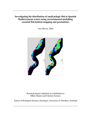
  • 1. Investigating the distribution of small pelagic fish in Spanish Mediterranean waters using environmental modelling, essential fish habitat mapping and geostatistics Alex Brown, 2006 Research project submitted in contribution to MRes Marine and Fisheries Science School of Biological Sciences (Zoology), University of Aberdeen, Scotland
  • 2. I declare that this thesis has been composed by myself and has not been accepted in any previous application for a degree. Information drawn from other sources and assistance received has been duly acknowledged. Signed: 21 August 2006 Alex Brown Date
  • 3. Acknowledgements I would like to acknowledge the provision of data and substantial contributions of time, effort, advice and hospitality of my primary supervisor, José Ma Bellido of the Centro Oceanográfico de Murcia (IEO), whom it was always a pleasure to work with. Thank you also to the many colleagues and friends who accomodated me in Murcia. I am very grateful to Vasilis Valavanis of the Hellenic Centre for Marine Research (HCMR) for providing data, accomodating me in Crete, and contributing many hours of patient guidance towards the completion of this project. My gratitude extends to Andreas Palialexis (HCMR) for his hospitality and technical advise. I also thank Colin MacLeod of the University of Aberdeen who invested considerable amounts of time and provided useful advice towards the completion of this project. Finally, I am grateful to Paul Fernandes of Fisheries Research Services, Aberdeen, for offering advice and providing me with the opportunity to participate in fieldwork related to this project.
  • 4. CONTENTS 1. INTRODUCTION 1 1.1 Environmental influences on the distribution of small pelagic fish 1.2 Essential Fish Habitat (EFH) 1.3 Geostatistics 1.4 Species ecology 1.5 Study area 1.6 Aims 2. METHODS 15 2.1 Survey data 2.2Allocation of zones 2.3 Environmental influences on the distribution of small pelagic fish 2.4 EFH mapping 2.5 Geostatistics 3. RESULTS 23 3.1 Environmental influences on the distribution of small pelagic fish 3.2 EFH mapping 3.3 Geostatistics 4. DISCUSSION 43 3.1 Environmental influences on the distribution of small pelagic fish 3.2 EFH mapping 3.3 Geostatistics 5. SUMMARY 51 REFERENCES 52 APPENDICES 57
  • 5. Brown, 2006 1 1. INTRODUCTION This study presents a multidisciplinary approach to investigating the distribution of small pelagic fish. For clarity and ease of reading, the study is presented in three main themes: environmental influences on the distribution of small pelagic fish, essential fish habitat (EFH) mapping and geostatistics. 1.1 Environmental influences on the distribution of small pelagic fish Small pelagic fish are predominantly confined to coastal regions, with the largest populations occurring in regions of upwelling. The spatial heterogeneity of the physical characteristics of the coastal pelagic environment, and the high mobility of small pelagic fish, generally leads to their distribution within areas which they find most favourable (Massé et al., 1996; Fréon et al., 2005). To a certain extent, fish show the ability to alter their behaviour in order to adapt to such a variable environment (Agenbag et al., 2003). However, all populations and species have an affinity for environmental conditions most favourable to their survival, growth and reproduction (review in Blaxter & Hunter, 1982). Fréon and Misund (1999) reviewed the environmental variables which have been related to the distribution of small pelagic fish (hereafter referred to only as ‘fish’). Temperature, salinity, dissolved oxygen, water transparency, light intensity, current, turbulence and upwelling, depth in the water column, bottom depth and substrate have all been shown to influence distribution at varying spatial and temporal scales. When studying environmental influences at a regional scale, variables with high spatial coverage are required. This places a major constraint on the environmental variables which can be used in the analysis (Agenbag et al., 2003), hence the dominant use of remotely sensed variables such as sea surface temperature (SST), sea surface chlorophyll-a concentration (Chl-a) and bathymetry. Using SST, an association between greater presence and abundance of fish and more mixed waters and thermal fronts has been observed for a number of species, including herring (Clupea harengus) in the northern North Sea (Maravelias & Reid, 1995);
  • 6. Brown, 2006 2 anchovy (Engraulis ringens) and sardine (Sardinops sagax) off the coast of Chile (Castillo et al., 1996); and sardine (Sardina pilchardus) and anchovy (Engraulis encrasicolus) in the northern Aegean Sea (Giannoulaki et al., 2005). However, such associations are commonly weak. Relationships between abiotic environmental factors (e.g. temperature and salinity) and fish distribution are likely to be indirect. In adult, non-spawning fish, the main factor influencing their distribution is prey. The vast majority of adult fish are planktivorous, and consume a combination of phytoplankton and zooplankton through filter or particulate feeding (Longhurst, 1971 in Blaxter & Hunter, 1982). Abiotic factors may provide an index for which biotic factors such as plankton abundance, which are more directly related to fish distribution (Mendelssohn & Cury, 1987; Maravelias & Reid, 1995; Agenbag et al., 2003). Associations between high concentrations of plankton and fish have been observed for C. harengus in the northern North Sea (Maravelias, 1999) and anchovy (Engraulis mordax) in the eastern Pacific (Robinson, 2004). At short time scales, environmental variability can change fish distributions with considerable fishery implications (Fréon et al., 2005). Rapid horizontal and vertical migrations can be induced, altering the distribution of fish and therefore their availability to fishing. While many of these shifts in distribution may be relatively local and temporary, they have been observed to persist for several months and over large areas, greatly influencing the exploitation of populations (Schwartzlose et al., 1999; Binet et al., 2001; Boyer et al., 2001; Bertrand et al., 2004). Schwartzlose et al. (1999) described the fishery implications of expansion and contraction of fish distribution. A larger area suitable for feeding and spawning may be beneficial to a fish population in terms of recruitment potential. However, an expansion in distribution will also alter their availability to fishing, possibly exposing them to more boats and dangerously high levels of fishing mortality. Conversely, the dispersion of a population over a greater area may reduce fishing mortality through increased difficulty in locating shoals. Contraction of distribution to a smaller area may make the population more
  • 7. Brown, 2006 3 available to those fleets which usually exploit them, and could be overexploited under certain management regimes. A wide range of methods for studying species distributions are now available including generalised linear models (GLMs) and generalised additive models (GAMs) (review in Guisan & Zimmermann, 2000). Both these techniques are frequently used to simultaneously test the roles of several environmental factors on species distribution (Guisan et al., 2002). GAMs use a link function to establish a relationship between the mean of a response variable and a smoothed function of the explanatory variable(s), and are able to deal with highly non-linear relationships, as are so often found in ecology (Hastie & Tibshirani, 1986, 1990 in Guisan et al., 2002). Many studies have used GAMs to study the distribution and abundance of marine species in relation to environmental conditions, including several species of small pelagic fish and cephalopods (e.g. Maravelias & Reid 1995; Bellido et al., 2001; Agenbag et al., 2003). As described by Barry & Walsh (2002), problems associated with zero-inflated data (as are commonly experienced with distribution data in ecology) can be avoided by separately modelling presence/absence and abundance given presence of species with the desired explanatory variables. 1.2 Essential Fish Habitat (EFH) The identification of EFH can be regarded as an application of studying relationships between fish distribution and the environment. The US Congress have defined EFH as ‘those waters and substrate necessary to fish for spawning, breeding, feeding, or growth to maturity’, including the physical, chemical and biological properties of the marine environment which support fish populations throughout their life cycle (DOC, 1997). EFH therefore consists of an array of habitat distributions corresponding to each life stage of a species. As described by Valavanis et al. (2004), habitat requirement information is needed for each life history stage, including the range of habitat and environmental variables with limiting effects on distribution.
  • 8. Brown, 2006 4 In a study on the distribution of short-finned squid (Illex coindetti) in the eastern Mediterranean Sea, Valavanis et al. (2004) used a Geographic Information System (GIS) based methodology of EFH mapping. A development of this technique is currently being applied to several sets of fishery data across the Mediterranean (including data used in this study) in the EC project ‘Environmental Approach to Essential Fish Habitat Designation’ (EnviEFH) (http://arch.imbc.gr/enviefh/). A combination of generalised additive models (GAMs) and GIS tools are used to analyse environmental preferences of species, then map EFH as areas of suitable environmental conditions. Where available, existing life history information on species distribution are used as constraints. The identification of EFH for commercial species may be used as a tool in spatial components of fisheries management. For example, by identifying areas of EFH, fisheries managers will be able to apply conservation measures to ensure the integrity of this EFH is sustained. For less mobile fish, and particularly those with important benthic habitat requirements, areas of EFH are likely to be fairly stationary over time. However, for highly mobile fish such as small pelagic species, stationary benthic features are of limited importance, particularly in non-spawning adults where feeding is the main activity (Fréon & Misund, 1999). As was described in section 1.1, environmental conditions such as temperature, salinity and plankton abundance are frequently important habitat properties for small pelagic fish. These conditions can show considerable spatio-temporal variability, therefore it is essential to identify EFH at regular intervals in order to monitor variability in both the quality and distribution of EFH. 1.3 Geostatistics Geostatistics refers to a variety of techniques for analysing the spatial structure of a resource. Initially developed for the exploitation of geological resources, geostatistics have been used in the study of fish populations since the late 1980s (Rivoirard et al.,
  • 9. Brown, 2006 5 2000). There are currently a wide range of techniques within the category of geostatistics, which have many potential applications (Kaluzny et al., 1998). In fisheries science, these techniques most frequently aim to quantify the level of spatial auto-correlation (clustering) within a fish population in order to provide a more accurate estimate of total abundance within a specified area (Maravelias et al., 1996; Maynou et al., 1998; Rivoirard et al., 2000). This study focuses on a combination of two complimentary tools which use sample data to analyse the spatial structure of a fish population in order to create an estimation of total abundance within a specified area. These are the variogram model and kriging, and are described in detail by Kaluzny et al. (1998). The variogram model The spatial structure of a fish population can be described by an empirical variogram, based on a variogram cloud. A variogram cloud is a scatterplot where each point is half the mean-squared difference in value z (e.g. fish density) between pairs of sample points separated by their geographic distance (h). The empirical variogram is a binned average of the variogram cloud where h, termed the ‘lag’, represents a value of distance ± half that distance (figure 1). As standard, empirical variograms are omni-directional, in that they consider differences between pairs of sample points in all directions. Before fitting a variogram model, several uni-directional empirical variograms must be produced which each consider differences only at certain orientations (e.g. 45°, 90°, 135°). If empirical variograms at different orientations are clearly very different in structure, fish shoals are directional in shape, and are said to be anisotropic. If anisotropy exists, it must be corrected for. If directional empirical variograms are all similar, no corrections need to be made and a model can be fitted to a standard omni-directional variogram.
  • 10. Brown, 2006 6 A variogram model is produced by fitting a line of a specified shape through the points of the empirical variogram. The line is fitted by minimising the residual sum of squares. From the variogram model, the parameters: nugget, sill, range and objective are obtained (figure 1). The nugget describes the amount of variance in z at very low distances. The sill is where the variogram levels off, and describes the maximum amount of variance in z. The range is the distance at which the sill is reached, and describes the distance at which correlation vanishes. The range may be interpreted as the approximate diameter of patches of fish. The objective is the residual sum of squares, and provides a measure of the goodness of fit between the variogram model and empirical variogram. Kriging Kriging is an interpolation technique for point data which creates predictions of a value (e.g. fish density) for a grid of specified points at a higher resolution than the sample points (Kaluzny et al., 1998). Predictions are based on the values at sampling points and the spatial structure of the fish population, as defined by the parameters nugget, sill and range from the variogram model. Kriging allows better visualisation of fish distribution, range sill nugget Figure 1. Empirical variogram (points) with spherical model fitted (black line), showing the parameters sill, nugget and range. X-axis = h (distance between sample points in nmi), y-axis = gamma (half the mean-squared difference in fish density (log)). Objective = residual sum of squares from spherical model.
  • 11. Brown, 2006 7 and potentially more accurate estimates of abundance than are provided by sample points alone. 1.4 Species ecology A variety of species of small pelagic fish are present in Spanish Mediterranean waters. They include sardine (Sardina pilchardus), anchovy (Engraulis encrasicolus), Mediterranean horse mackerel (Trachurus mediterraneus), Atlantic horse mackerel (Trachurus trachurus), round sardinella (Sardinella aurita), bogue (Boops boops), chub mackerel (Scomber japonicus) and Atlantic mackerel (Scomber scombrus) (Giráldez, 2005). Although all of these species are caught by commercial fisheries, sardine and anchovy have traditionally been the most commercially important (Pertierra & Lleonart, 1996), and have therefore been the main focus of scientific studies. A common feature of the distribution of clupeoids such as sardine and anchovy is their association with upwelling systems, productive bays and estuaries, or shallow, productive continental shelves (Blaxter & Hunter, 1982). The productivity of these environments in the western Mediterranean is initiated by hydrological processes such as river run-off, upwelling of deep/slope waters to the surface, and mixing within the water column (Estrada, 1996). These processes bring nutrient rich waters into the photic zone, allowing phytoplankton growth. In the Mediterranean Sea, zooplankton abundance and distribution are positively correlated with phytoplankton development (Champalbert, 1996). Studies on the ecosystem functioning of the northwest Mediterranean have shown pelagic species to dominate the total biomass, catches, and account for the greatest number of flows between trophic levels (Tudela & Palomera, 1997; Coll et al., 2006). Sardine, anchovy, and several other planktivorous small pelagic species play a major role in western Mediterranean ecosystems by channelling energy from low to higher trophic levels (Tudela & Palomera, 1997).
  • 12. Brown, 2006 8 Both sardine and anchovy are planktivorous, usually feeding on a combination of phytoplankton and zooplankton through filter-feeding and selective consumption of larger prey (Blaxter & Hunter, 1982). A greater proportion of zooplankton is consumed by anchovies than sardine (Louw et al., 1998), and studies on spawning aggregations of anchovy in both the Gulf of Lions and Gulf of Valencia have shown a clear dominance of copepod zooplankton in their diet (Tudela & Palomera, 1997; Plounevez & Champalbert, 2000). In the western Mediterranean, anchovy spawn and are mainly caught in spring and summer when the majority of individuals are 1 year old (Palomera, 1992; Pertierra & Lleonart, 1996). Sardine spawning extends from October to May, with a peak during winter (Olivar et al., 2001), while they are caught mostly in the spring and autumn when the majority of individuals are between 1 and 2 years old (Lloret et al., 2004). Temperature preferences for spawning are between 15-22°C for anchovy (García & Palomera, 1996) and below 20°C, with increased intensity below 18°C, for sardine (Olivar et al., 2003). The temperature preferences of adult anchovy and sardine in the western Mediterranean are undocumented outside of spawning events. However, in the northern Aegean Sea Giannoulaki et al. (2005) showed non-spawning sardine to occupy warmer waters than spawning anchovy, with the suggestion that warmer waters provided favourable conditions for somatic growth. 1.5 Study Area The study area comprises the entire Mediterranean coast of Spain. This extends from the southern Gulf of Lions in the north, through the Gulf of Valencia to the south, before ending at the Strait of Gibraltar in the western Alboran Sea (figure 2). A study area boundary is defined to encompass the continental shelf (to 200m depth contour) environment (coastline to 200m depth contour) and a small area immediately offshore of this.
  • 13. Brown, 2006 9 The Mediterranean Sea is generally considered an area of low, but fairly stable productivity (Margalef, 1985). However, many areas of higher productivity exist where oceanographic and meteorological conditions are favourable for primary productivity (Lloret et al., 2004). Several such features have been identified in the Spanish Mediterranean. The Gulf of Lions and Gulf of Valencia In the north, the Gulf of Lions is a well documented region of high productivity, caused by a combination of a fairly wide continental shelf; considerable river run-off from the Rhône; and a high degree of wind-induced mixing and upwelling from the strong, predominantly north-westerly winds blowing in this region (Estrada, 1996; Salat, 1996; Figure 2. The study area and its surrounding geography. Including nearby cities and major rivers draining into the study area.
  • 14. Brown, 2006 10 Agostini & Bakun, 2002). Slightly to the south, fertilization of Catalan shelf waters is caused by local vertical mixing and intrusions of slope waters onto the shelf through submarine canyons (Salat et al., 2002). The influence of these processes in the Gulf of Lions and Catalan shelf extend south along the Spanish coast through the passage of the Northern Current. Also known as the Liguro-Provencal-Catalan Current, the Northern Current flows in a south west direction along the continental slope from the Gulf of Genoa to the Gulf of Valencia (figure 3) (Millot, 1987 in Millot, 1999; Font et al., 1995). Fresh, nutrient enriched waters from the rivers Rhône and Ebro become entrained in the Northern Current, producing a shelf/slope haline front between the less saline coastal waters and more saline offshore water (Font et al., 1995). The Northern Current exhibits increased strength and mesoscale activity during winter months due to greater wind forcing (Millot, 1999). In the Gulf of Valencia, the wide Iberian shelf deflects the Northern Current further offshore. Here, coastal waters are more influenced by local Figure 2. The path of the Northern Current along the continental slope of the north-western Mediterranean. Source: Font et al. (1995).
  • 15. Brown, 2006 11 meteorological events and freshwater inputs (Salat, 1996). Salat et al. (2002) suggested that nutrient inputs from the Ebro outflow may account for 10-25% of the total nutrient content in the waters of the adjacent Iberian shelf. In addition to riverine inputs in this area, nutrient enrichment also occurs around the Ebro delta as a result of intense water mixing on the wide shelf, induced by the strong north-westerly winds associated with this region (Estrada, 1996; Salat, 1996). Regional enrichment events such as those described above have been shown to greatly influence the productivity and fishing activity associated with anchovy on the Iberian shelf (Palomera, 1992; Agostini & Bakun, 2002; Lloret et al., 2004). The Gulf of Lions and Iberian shelf around the Ebro delta are the main spawning areas of anchovy in the northwest Mediterranean (García & Palomera, 1996). They also provide important sardine spawning habitats (Olivar et al., 2001). The prevalence of sardine and anchovy in these waters is confirmed by a high level of fishing activity, where pelagic trawl and purse seine techniques yield some of the highest landings of these species in the Mediterranean (Pertierra & Lleonart, 1996). The Alboran Sea In addition to the Gulfs of Lions and Valencia, the Alboran Sea is another well documented area of productivity within the western Mediterranean. Agostini & Bakun (2002) identified the Alboran Sea, along with the Gulf of Lions and adjacent Catalan coast, as two of five ‘ocean triad’ regions in the Mediterranean. Ocean triads are defined as areas of high productivity, with enrichment, concentration and retention processes favourable for reproduction and growth in coastal pelagic fishes (Bakun, 1998). Wind-driven processes of nutrient enrichment are less intense in the Alboran than the north-west Mediterranean (Agostini & Bakun, 2002), the continental shelf is very narrow, and there are no major river inputs. Instead, the input of cooler, less saline, nutrient rich Atlantic surface water at the Strait of Gibraltar dominates the hydrographic characteristics of the region. A ‘jet’ of Atlantic water causes turbulent mixing in the
  • 16. Brown, 2006 12 Strait, and the development of two anticyclonic gyres in the Alboran Sea (figure 4) with associated upwelling on the Spanish coast (Tintorè et al., 1991; Estrada, 1996). All of these processes cause areas of enhanced primary productivity and corresponding high zooplankton concentrations along the Spanish Alboran coast (Estrada, 1996; Champalbert, 1996; Viudez et al., 1998). Along with the Gulf of Lions and Iberian shelf, the Alboran Sea represents an important area of anchovy concentration and fishing in the western Mediterranean (Garcia & Palomera, 1996). The Bay of Málaga has been identified as an anchovy and sardine nursery ground, and the transport of eggs and larvae into the Mediterranean from spawning grounds in the Atlantic has been shown (García & Palomera, 1996). Costa Blanca and Golf of Vera There is little mention in the scientific literature of the oceanographic processes taking place in the Costa Blanca and Gulf of Vera. These regions form something of a transition zone between the influence of the Northern Current in the north, and the Algerian current in the Alboran Sea (Millot, 1999). The continental shelf is very narrow in the Gulf of Vera and there are no major freshwater inputs into the area. The latter is also true of the Costa Blanca, as discharge from the River Segura is minimal (Bellido, pers. comm.). However, the continental shelf is fairly wide, and it is likely that this region is somewhat Figure 4. Circulation in the Alboran Sea, showing Western and Eastern Alboran Gyres (WAG and EAG respectively), and the associated Algerian Current. Source: Baldacci et al. (2001).
  • 17. Brown, 2006 13 influenced by processes further north (Millot, 1987 in Millot, 1999). Anchovy catches are traditionally low in the Gulf of Vera region (García & Palomera, 1996). 1.6. Aims This study aimed to use a GIS-based environmental modelling approach to investigate relationships between the distribution and abundance of small pelagic fish and environmental conditions in Spanish Mediterranean waters. A further aim was to apply an extension of this approach to sardine and anchovy specifically, in order to identify EFH and its temporal variability. Finally, geostatistics were to be used to further investigate the distribution and abundance of fish. These aims were achieved by undertaking the following specific tasks: Environmental influences on the distribution of small pelagic fish 1. Develop a GIS for the purpose of storing, integrating, processing and visualising survey and environmental data. 2. Model relationships between the presence/absence of fish and environmental conditions for each zone and year, using only the presence/absence of fish. 3. Model relationships between abundance of fish and environmental conditions for each zone and year, using data only where fish are present. EFH mapping 4. Repeat task 2 but using the presence/absence of sardine and anchovy, rather than small pelagic fish in general, and only for all years combined. 5. Select models produced in task 4, and use these to predict the probability of presence of sardine and anchovy throughout the study area in each year.
  • 18. Brown, 2006 14 6. Using predictions from task 5, produce maps to visualise the spatial distribution of EFH. 7. Analyse spatial and temporal trends in the distribution and quality of EFH between years. Geostatistics 8. Process acoustic data to obtain values of fish density per nmi2 for use in geostatistical analyses. 9. Using values of fish density obtained in task 8, produce variogram models to analyse the spatial structure of sardine and anchovy distributions in each zone and year. 10. Based on the variogram models produced in task 9, perform kriging to interpolate values of fish density to a higher resolution than that of the survey data. Then, use kriged values to estimate the total abundance of fish throughout the study area.
  • 19. Brown, 2006 15 2. METHODS 2.1 Survey Data Biological data were collected by the Instituto Español de Oceanografía (IEO) aboard the Research Vessel Cornide de Saavedra during annual acoustic surveys. The surveys began in the north at the France/Spain border (42.42°N, 3.43°E) in the penultimate week of November, before progressing south and east to finish at the Strait of Gibraltar (36.13°N, 5.26°W) approximately 4 weeks later. The entire Spanish Mediterranean coast is surveyed in a total of 128 individual transects covering a distance of 1270 nautical miles (nmi). Transects are oriented perpendicular to the coast and parallel to each other, with the intention of surveying the continental shelf between the 30m and 200m isobaths (figure 4). Transect length was a minimum of 5 nmi, so the survey extended slightly beyond the 200m isobath in areas of extremely narrow continental shelf. Transects were separated by 4 nmi in areas where the continental shelf is narrow (zones 1 and 3), and 8 nmi where the shelf is wide (zone 2). Acoustic equipment comprises a SIMRAD EK-500 scientific echosounder operating at 38 KHz with a split beam transducer, and an additional SIMRAD EY-500 echosounder. The echosounders were calibrated prior to commencing each survey in accordance with the standard 60mm copper sphere method (Foote et al., 1987). Acoustic signals were integrated into Elementary Distance Sampling Units (EDSUs) for every 1 nmi surveyed. Acoustic signals were later processed using Sonar Data’s Echoview software to remove signals not attributable to fish, and give a total Nautical Area Scattering Coefficient (NASC) value per EDSU. NASC describes m2 of cumulative backscattering cross section per nmi2 , and is considered a measure of abundance in this study. A species composition was assigned to each NASC based upon experimental fishing in the vicinity of the EDSU (as described in MacLennan and Simmonds, 1992). Acoustic surveying took place between the hours of 06:00 and 18:00, with experimental fishing at night. The surveys described above generated 1290, 1292 and 1268 records for 2003, 2004 and 2005 respectively with almost exact spatial overlap between years. Each record describes
  • 20. Brown, 2006 16 the central longitude and latitude, NASC and species composition of each EDSU. For the years 2004 and 2005, data were also available describing the mean length frequency distribution of each species for the total survey area (obtained through experimental fishing). This allowed the calculation of fish density from NASC for these two years. 2.2 Allocation of zones The study area was divided into 3 zones, which were considered throughout all analyses (figure 5). As described in section 1.5, oceanographic and fishery characteristics vary considerably throughout the study area, and therefore it is sensible to consider fish – environment relationships at different spatial scales. For geostatistical purposes, the boundaries of zones are defined according to inter- transect distance used in the survey. Zones 1 and 3 are areas of fairly narrow continental shelf where transects are separated by 5 nmi, in contrast to the 8 nmi spacing in zone 2. Consistent inter-transect spacing is advisable when considering the spatial structure of fish assemblages (Rivoirard et al., 2000) Figure 5. Map showing the extent of zones 1 (blue), 2 (red) and 3 (green), and transects locations (black lines).
  • 21. Brown, 2006 17 In addition to geostatistical considerations, differences in the geography and oceanography of the Spanish Mediterranean coast are well represented by these zones. Zone 1 faces predominantly east and south east, and is influenced by the Northern Current and processes taking place in the Gulf of Lions. Zone 2 faces predominantly south east, and is dominated by the wide Iberian shelf and its associated hydrological features. Zone 3 is an area of extremely narrow continental shelf, with the south facing Alboran coast influenced by inflow of Atlantic waters, and the south east facing Gulf of Vera representing a transition zone between southern and northern hydrographic processes. 2.3 Environmental influences on the distribution of small pelagic fish GIS development and environmental data A GIS was developed using Environmental Systems Research Institute’s ARC/INFO and ArcView 3.3 software. A large number of environmental data were collated from internet-based sources by the Hellenic Centre for Marine Research1 , then processed into files suitable for use in a GIS (table 1). These data overlapped temporally with the dates of surveys (November and December 2003, 2004 and 2005). The spatial resolution of these data varied from one source to another, so all were converted to the same resolution as sea surface temperature (which had the highest resolution) using the ‘Topogrid’ interpolation function in ARC/INFO. Point covers of fisheries records were combined with environmental grids to extract environmental values for each fisheries record. Care was taken to ensure the temporal resolution of the environmental grid matched that of the fisheries sampling date. Maps were produced to visualise the distribution of NASC values throughout the study area. 1 Hellenic Centre for Marine Research, Crete, Greece. www.hcmr.gr
  • 22. Brown, 2006 18 Variable Units Source Sensor/Model URL Photosynthetically Active Radiation (PAR) (E/m2 /d) Oceancolor WEB, GSFC/NASA, USA SeaWiFS http://oceancolor.gsfc.nasa.gov Sea Level Anomaly (ALT) cm Live Access Server, Merged (TOPEX/Poseidon, Jason-1, ERS-1/2, Envisat) http://www.aviso.oceanobs.com/ Sea Surface Temperature (SST) °C DLR EOWEB, Germany AVHRR SST http://eoweb.dlr.de:8080/ Sea Surface Chlorophyll-a Concentration (Chl-a) (mg/m3 ) Oceancolor WEB, GSFC/NASA, USA SeaWiFS http://oceancolor.gsfc.nasa.gov Sea Surface Salinity (SSS) psu IRI/LDEO, USA CARTON-GIESE SODA and CMA BCC GODAS http://ingrid.ldeo.columbia.edu/ Wind Speed (WS) (m/sec) RS Systems, USA QuikSCAT http://www.ssmi.com/ Wind Direction (WD) (° from N) RS Systems, USA QuikSCAT http://www.ssmi.com/ Bathymetry (depth) m NGDC, NOAA, USA Geostat ERS-1 satellite & ship depth echosoundings http://www.ngdc.noaa.gov/mgg/ image/2minrelief.html Table 1. Sources and descriptions of environmental data used in the GIS
  • 23. Brown, 2006 19 Generalised Additive Models (GAMs) Despite having a choice of 8 different environmental variables to use as explanatory variables in GAMs (hereafter referred to as ‘models’), it was decided that many were unsuitable for this type of model. For example, there was collinearity amongst several of the variables, and some showed very little variability throughout the study area (eg. SSS, WS, WD). SST, Chl-a and depth were selected for models as they showed considerable variability and were believed to be easier to interpret biologically than some other variables available. To overcome problems associated with the zero-inflated nature of our data, a two-stage modelling process was used as suggested in Barry & Welsh (2002). Firstly, only the association between presence/absence of fish and the environmental variables was modelled. In the second step, only records with species presence were used so that the association between NASC and environmental variables could be modelled. Modelling procedure Highland Statistic Ltd’s ‘Brodgar’ interface for ‘R’ was used to carry out the modelling. Models were produced for both the entire survey area, and for each of the three zones described in section 3.2. This was done for each year individually, in addition all years combined. For presence/absence models, a binomial or quasibinomial (where the overdispersion parameter exceeded 1.0) distribution and logit link function were used. In models using NASC as a response variable, a poisson distribution and log link function were used. All environmental variables were used as smoothing terms. Due the presence of several extreme values, a natural log transformation was applied to SST, Chl-a, depth and NASC.
  • 24. Brown, 2006 20 For each model, a forward step-wise selection method was used to select the combination of environmental variables which produced the best model in terms of the lowest possible AIC. The deviance explained and significance of each variable was noted, but did not influence the choice of model. Where collinearity existed between variables, they were modelled separately before selecting the variable which produced the best model. Cross validation was applied during modelling to estimate the optimum number of degrees of freedom of each smoother. Classification trees (for presence/absence) and regression trees (for NASC) were produced for each combination of variables in the best models. This allowed the relative importance of each variable in a model to be calculated. The detailed properties of trees were not considered in the analyses. 2.4 EFH mapping As sardine and anchovy have traditionally been the most economically important species in the Spanish Mediterranean (Pertierra & Lleonart, 1996), they were both chosen for EFH mapping. The GAM procedure described in section 2.3:’modelling procedure’ was repeated using presence/absence data for sardine and anchovy, although models were only produced using all years combined – not individual years. Through the GIS, boundaries were defined to encompass the surveyed points and the surrounding area. Within each boundary, point values were extracted from each of the environmental data grids and merged into spreadsheet files, providing high resolution data of the environmental conditions in each year. Using the statistical package R, presence/absence models were used to predict the probability of species presence for the aforementioned high resolution environmental data. The predictions were then mapped as grids. Once the probability of species presence was predicted for the entire area, both species and each year, the characteristics of these predictions were analysed. Scatterplots comparing predictions between years provided qualitative visual analysis of inter-annual differences in predictions at specific locations. Cumulative frequency plots enabled the
  • 25. Brown, 2006 21 comparison of predictions for an entire area. Kolmogorov-Smirnov (KS) tests were used to statistically quantify differences in the frequency distribution of predictions between years. 2.5 Geostatistics Data processing Spreadsheets were developed to convert the NASC of each record into fish density for each species, as no existing conversion tools were designed to deal with either this volume of data or number of species. As with EFH mapping, only sardine and anchovy were selected for geostatistical analysis. However, it was essential to calculate fish density of all species in order to accurately apportion the NASC between species. A target strength of 20log(L) -71.9 (where L is the fish length (cm) and -71.9 is a constant) was used for all species. Target strengths estimates have been shown to vary between different species of similar fish, between different areas, and according to the size range of fish considered (review in Simmonds & MacLennan, 2005). However, in the absence of calculated target strengths for any of the species surveyed in this area, the value of 20log(L) -71.9 seemed most appropriate as it is based on calculations from a variety of clupeoid fishes of many length classes in a variety of areas (Foote, 1987 in Simmonds & MacLennan, 2005). It was decided that, based on target strength information available, this value would be the least likely to cause large errors in abundance estimates of any one species. The variogram model All geostatistical analysis was performed using Insightful’s S-PLUS software package with Spatial Stats module, following the methods described in Kaluzny et al. (1998). Variograms used fish density data, and were produced for each species, zone and year. Units of longitude and latitude were converted from decimal degrees to x and y co-
  • 26. Brown, 2006 22 ordinates in nmi. For empirical variograms, the lag was specified as 1 nmi greater than the inter-transect distance for zones 1 and 3, and 2 nmi greater than the inter-transect distance for zone 2. This allowed the variograms to consider differences in fish density between neighbouring transects. Multi-directional empirical variograms confirmed an absence of anisotropy for all species, zones and years. Omni-directional empirical variograms were fitted with spherical models (appendices 19 – 20). The fit was optimized through minimizing the residual sum of squares. The variogram model provided the parameters nugget, sill and range for each species, zone and year. Kriging Polygons were manually defined for each zone to encompass the surveyed points. New sampling grids with a resolution of 1 nmi2 were defined within each polygon. Using the parameters obtained from variogram models described above, ordinary kriging was performed on the surveyed fish density values. This produced predicted values of fish density for the new sampling grid which could be mapped in the GIS. As the units of fish density were fish nmi-2 , and the resolution of kriged predictions was 1 nmi2 , the sum of fish density data per zone provided estimates of total abundance.
  • 27. Brown, 2006 23 3. RESULTS 3.1 Environmental influences on the distribution of small pelagic fish Visualising the distribution of NASC The mapping of NASC values for each zone and year allowed visualization of spatial and temporal trends in the distribution of fish (figures 6-8). The addition of a layer displaying Chl-a allowed the distribution of fish to be visualised relative to this environmental variable. In zone 1, there are two main areas where the greatest NASC values were found (figure 6). One of these areas existed at the northern limits of the survey, in the southern Gulf of Lions where the coast faces east. This area also showed some of the highest Chl-a in the zone. NASC values in this area were highest in 2003. Another zone of consistently high NASC existed north and south of Barcelona, also where higher Chl-a was seen. Again, 2003 showed the highest values of NASC. In zone 2, high NASC values were most abundant in the north, where the continental shelf is wide and Chl-a was generally high (figure 7). A peak in Chl-a existed around the delta of the River Ebro, but high NASC values were not restricted to this area. South of the Gulf of Valencia, along the Costa Blanca, several locations showed a high NASC, although these were patchier in distribution than in the north. NASC values were noticeably lower in 2004 compared to other years. In zone 3, high NASC values were seen almost all along the narrow continental shelf (figure 8). These were most consistent in the western Alboran Sea, which was also an area of high Chl-a. In 2005, notably higher Chl-a was seen in the Gulf of Vera. Interestingly, a small area of very high Chl-a showed a complete absence of fish. NASC values were generally lower in 2004 compared to other years
  • 28. Brown, 2006 24 2003 2004 2005 Figure 6. Zone 1 NASC and Chl-a for 2003 – 2005.
  • 29. Brown, 2006 25 2004 2003 2005 Figure 7. Zone 2 NASC and Chl-a for 2003 – 2005.
  • 30. Brown, 2006 26 Figure 8. Zone 3 NASC and Chl-a for 2003 – 2005. 2003 2004 2005
  • 31. Brown, 2006 27 Presence/Absence Data The proportion of records with fish presence showed considerable spatial and temporal variation (table 2). 2005 yielded the highest proportions of fish presence, 2004 the lowest, with 2003 slightly higher than 2004. Generally, zone 1 showed the highest proportions of fish presence, with zone 2 slightly lower, and zone 3 the lowest. There were some exceptions to this trend, particularly zone 1, 2003, which exhibited a lower proportion of presence than the general trend suggests. Year Zone Records with fish present/absent Proportion with fish present 2003 All 1 2 3 658 / 632 137 / 155 360 / 301 161 / 337 0.510 0.469 0.545 0.478 2004 All 1 2 3 603 / 689 152 / 149 310 / 352 141 / 188 0.467 0.505 0.468 0.429 2005 All 1 2 3 778 / 490 201 / 99 414 / 236 163 / 155 0.614 0.670 0.637 0.513 All All 1 2 3 2039 / 1810 490 / 403 1084 / 889 465 / 518 0.530 0.549 0.549 0.473 GAMs were able to explain between 21.3% and 51.5% of the deviance in fish presence/absence (table 3). Some common trends in these results were apparent. Models for zone 1 explained the least deviance, followed by models for all zones combined. Generally, the greatest proportion of deviance was explained by models for zone 3. However, in 2005, the model for zone 2 explained the most deviance. When considering all zones combined, the greatest proportion of deviance was explained by the model for 2005, followed by 2003, then all years combined, and then 2004. Table 2. Presence/absence of fish records for each zone and year, including the proportion of records with fish present
  • 32. Brown, 2006 28 In all models, depth was the most important variable and was always highly significant. The relationship between depth and fish presence/absence was generally strongly negative with increasing depth, although a few models did show fluctuations in this trend at more shallow depths (appendices 1 - 4). For the majority of models, depths in excess of approximately 100m (4.6 on natural log scale) had a negative effect on fish presence. Another common characteristic was a small peak in the positive influence of depth on fish presence between approximately 35 – 60m (3.5 – 4.1 on natural log scale) (figure 9). Chl-a was frequently the second most important variable, and was significant in all models except zones 1 and 2 in 2004. The relationship between fish presence/absence and Chl-a was fairly weak and positive, with increasing chlorophyll-a concentration generally leading to greater fish presence. At very high Chl-a, the relationship was subject to considerable uncertainty due to a low number of values (figure 9). SST was the least frequently used variable, although it was still included in 11 of the 16 models produced. It was generally the least important variable, and was often non- significant. However, it was more important than Chl-a in 3 out of 4 models for zone 3. Whenever co-linearity existed between Chl-a and SST, chlorophyll was always the more important of the two variables. The character of the relationship between SST and fish presence/absence varied spatially and temporally, and was generally very weak. In zone 3, there was a negative relationship between increasing SST and fish presence. In other zones, the relationship often showed a peak in positive influence on fish presence between approximately 16°C and 17°C (2.77 – 2.83 on natural log scale) (figure 9).
  • 33. Brown, 2006 29 Year Zone n Variables (p-value) Deviance Explained (%) 2003 All 1 2 3 1290 292 661 337 depth (<0.01), Chl-a (<0.01), SST (0.23) depth (<0.01), Chl-a (<0.01), depth (<0.01), Chl-a (<0.01), SST (0.40) depth (<0.01), SST (<0.01) 32.6 21.3 35.7 50.1 2004 All 1 2 3 1292 301 662 329 depth (<0.01), Chl-a (<0.01) depth (<0.01), Chl-a (0.08), SST (<0.01) depth (<0.01), Chl-a (0.07) depth (<0.01), Chl-a (<0.01) 29.3 26.5 30.6 44.1 2005 All 1 2 3 1268 300 650 318 depth (<0.01), SST (<0.01) depth (<0.01), Chl-a (<0.05) depth (<0.01), Chl-a (<0.05), SST (<0.01) depth (<0.01), SST (0.78), Chl-a (<0.05) 39.7 33.4 51.5 48.7 All All 1 2 3 3849 893 1973 983 depth (<0.01), Chl-a (<0.01), SST (<0.01) depth (<0.01), Chl-a (<0.01), SST (<0.01) depth (<0.01), Chl-a (<0.01), SST (<0.01) depth (<0.01), SST (<0.01), Chl-a (<0.01) 32.3 24.5 36.3 45.3 Table 3. Fish presence/absence GAM results, showing the best model for each zone and year. Variables are ordered according to their importance in the model, based on results from classification trees. The order runs from left (most important) to right (least important). Non-significant variables are highlighted in red.
  • 34. Brown, 2006 30 Figure 9. Fish presence/absence GAM plots, all years combined. X-axis = explanatory variable used as a smoother (natural log scale), depth (left), Chl-a (middle), SST (right). Y-axis = influence of smoother on the presence of fish. Dashed lines represent 95% confidence interval. Fish presence/absence GAM plots, all years combined Zone 3 Zone 2 Zone 1 All zones combined
  • 35. Brown, 2006 31 NASC Data GAMs were able to explain between 2.03% and 16.2% of the deviance in NASC (table 4). When considering all zones combined, the greatest proportion of deviance was explained by the model for 2005, followed by 2003, then all years combined, then 2004. This was the same trend as was seen using presence/absence data. However, when considering individual zones, models for zones 1 and 2 in 2005 explained the least deviance of all years, whereas zone 3, 2005 explained the most. The choice of variables used in models varied considerably both spatially and temporally, with no obvious consistent trends between years or zones. Depth was the most frequently used variable, included in 13 of the 16 models, followed by SST (8 out of 16 models), then Chl-a (6 out of 16 models). Chl-a was not used in any models for 2005, and SST was only used in 2005 for all zones combined. Where depth was used, it showed a negative relationship with NASC, similar to that between depth and fish presence/absence, although the relationship with NASC more weak. The influence of depth on fish presence became negative at depths in excess of approximately 60m (4.1 on natural log scale) (figure 10, and appendices 5 - 8). The relationship between Chl-a and NASC was similarly positive to that of chlorophyll and fish presence/absence, with increasing Chl-a showing an increasingly positive effect on NASC (figure 10, and appendices 5 - 8). As with presence/absence models, this relationship was generally weak, and there was considerable uncertainty in this relationship at very high Chl-a due to a low number of values. The character of the relationship between SST and NASC varied spatially and temporally, and was often weak. In all zones combined and zone 3, there was a negative relationship between increasing SST and NASC. For zone 1, there was a weak positive relationship between SST and NASC, although this was non-significant in all years.
  • 36. Brown, 2006 32 Year Zone n Variables (p-value) Deviance Explained (%) 2003 All 1 2 3 658 137 360 161 Chl-a (<0.01), depth (0.09), SST (<0.05) Chl-a (<0.01), SST (0.15) SST (<0.01) , depth (0.46) depth (0.07) 11.3 12.6 14.1 2.81 2004 All 1 2 3 603 152 310 141 depth (<0.05), Chl-a (<0.05) depth (<0.01), SST (0.56) Chl-a (<0.01) SST (0.26) 6.13 14.1 5.65 2.83 2005 All 1 2 3 778 201 414 163 SST (<0.01), depth (0.20) depth (0.35) depth (<0.01) depth (<0.01) 16.2 2.03 4.16 5.43 All All 1 2 3 2039 490 1084 465 Chl-a (<0.01), depth (<0.01), SST (0.12) depth (<0.01) depth (<0.01), Chl-a (<0.05), SST (0.15) SST (<0.01), depth (0.15) 7.65 4.89 7.46 10.3 Table 4. NASC GAM results, showing the best model for each zone and year. Variables are ordered according to their importance in the model, based on results from regression trees. The order runs from left (most important) to right (least important). Non- significant variables are highlighted in red.
  • 37. Brown, 2006 33 Figure 10. NASC GAM plots, all years combined. X-axis = explanatory variable used as a smoother (natural log scale), depth (left), Chl-a (middle), SST (right). Y-axis = influence of smoother on the NASC. Dashed lines represent 95% confidence interval. NASC GAM plots, all years combined Zone 3 Zone 2 Zone 1 All zones combined Variable not used Variable not used Variable not used
  • 38. Brown, 2006 34 3.2 EFH Mapping GAMs revealed relationships between the presence/absence of sardine and anchovy and environmental conditions (appendices 9 - 11). The characteristics of these relationships are not discussed in detail here, but they can be described as generally similar to those identified in section 3.1:’presence/absence data’ between fish presence/absence and environmental conditions. For sardine, models explained 23.9%, 36.3% and 40.3 % of the deviance for zones 1, 2 and 3 respectively (appendix 9). For anchovy, models explained 26.5%, 37.2% and 33.6 % of the deviance for zones 1, 2 and 3 respectively (appendix 9). All models used depth, SST and Chl-a, except anchovy, zone 3, which did not use SST. Mapping of the predictions allows visual analysis of the distribution and quality of fish habitat (figure 11, and appendices 12 - 13). In this study, EFH is not defined as habitat with a predicted probability of presence above a specific threshold value. Instead, all areas within the study area are referred to as EFH, with comparisons being made in accordance with the quality of this EFH. Higher predictions clearly indicate better quality habitat, in terms of the environmental variables considered in the model on which the predictions are based. Zone 1 showed the greatest inter-annual variation in the quality of EFH (figure 11). For both species, areas of high predictions were similar to those of higher NASC values as described in section 3.1: ‘visualising the distribution of NASC’. These included the southern Gulf of Lions and areas north and south of Barcelona. 2005 clearly showed the highest predictions, which were also the most widespread high predictions of all the years. 2003 showed fairly high predictions in the southern Gulf of Lions and south of Barcelona, but low predictions north of Barcelona. In 2004, the habitat appeared to be of good quality around Barcelona, but there were very low predictions in the southern Gulf of Lions. This was most apparent for anchovy, where a probability of presence was rarely predicted above 0.3 in this area.
  • 39. Brown, 2006 35 Sardine, 2003 Sardine, 2004 Sardine, 2005 Anchovy, 2003 Anchovy, 2004 Anchovy, 2005 Figure 11. EFH maps showing the predicted probability of presence of sardine and anchovy in zone 1 for 2003, 2004 and 2005.
  • 40. Brown, 2006 36 Inter-annual trends in the quality of EFH were further analysed through cumulative frequency plots (figure 12) and scatterplots (figure 13). KS tests quantified inter-annual differences in the frequency distributions of EFH predictions (table 5). Cumulative frequency plots showed zone 1 to exhibit the greatest inter-annual differences in EFH (figure 12, and appendix 15). In this zone, the same trend in differences was apparent for both sardine and anchovy, although differences were of a greater magnitude for anchovy. While the quality of EFH in years 2003 and 2004 appeared similar, 2005 was quite different. A cumulative frequency of 1 was reached at a much higher predicted probability of presence in 2005. This indicated a greater proportion of higher predictions in 2005, particularly for predictions in excess of approximately 0.7 – where the graph steepened. KS tests calculated the maximum difference between the cumulative frequencies of predictions in each year (KS-value), and the significance of these differences (table 5). KS-values were greater for anchovy than sardine in all zones and between all years (with the exception of zone 2, 2004 vs 2005, where values were the same for both species). KS- values were generally greatest in zone 1, then zone 3, with zone 2 showing the lowest values. Zone 2 also showed the most consistent KS-values between the different pairs of Zone 1, Sardine 0 0.2 0.4 0.6 0.8 1 0.0 0.2 0.4 0.6 0.8 1.0 Predicted probability of presence Cumulativefrequency 2003 2004 2005 Zone 1, Anchovy 0 0.2 0.4 0.6 0.8 1 0.0 0.2 0.4 0.6 0.8 1.0 Predicted probability of presence Cumulativefrequency 2003 2004 2005 Figure 12. Cumulative frequency of predicted probability of presence for sardine (left) and anchovy (right) in zone 1.
  • 41. Brown, 2006 37 years compared. All KS-values were said to be significant, although this is likely to be an artefact of the high number of samples and is of no real use in quantitative comparisons. Zone n Years compared Sardine KS value Sardine P-value Anchovy KS value Anchovy P-value 1 5137 2003 vs 2004 2003 vs 2005 2004 vs 2005 0.0493 0.1901 0.1551 <0.05 <0.05 <0.05 0.1513 0.2251 0.2391 <0.05 <0.05 <0.05 2 16702 2003 vs 2004 2003 vs 2005 2004 vs 2005 0.0808 0.0752 0.0743 <0.05 <0.05 <0.05 0.1011 0.0868 0.0743 <0.05 <0.05 <0.05 3 7013 2003 vs 2004 2003 vs 2005 2004 vs 2005 0.0503 0.0884 0.1199 <0.05 <0.05 <0.05 0.0627 0.1636 0.1439 <0.05 <0.05 <0.05 While cumulative frequency plots showed differences in EFH for the entire zone as a whole, scatterplots (figure 13, and appendices 16 - 18) showed differences in EFH by comparing predictions at exact locations within each zone. Where a point is above the red line, the prediction for the y-axis year was greater than the prediction for the x-axis year at the same location. Where a point is below the red line, the prediction for the y-axis year was less than the prediction for the x-axis year at the same location. The greater the vertical distance between the point and the red line, the greater the difference in prediction between the two years. Scatterplots generally showed smaller differences in predictions between years at lower predicted values, suggesting that locations with low predicted probability of presence remain consistently low between years. Similarly, higher predicted values showed fairly low differences between years. This could be due to the influence of depth in the models Table 5. Results of KS tests. The number of values in each zone (in any one year) is given as n. KS values provide a measure of the maximum difference between frequency distributions of predictions between years. The significance of each KS value is shown by its corresponding p-value
  • 42. Brown, 2006 38 Figure 13. Scatterplots comparing predicted probability of presence between years. Both axis show the predicted probability of presence for the year they are labelled with. The red line is drawn manually for visual reference purposes only – it is not a trend line.
  • 43. Brown, 2006 39 used to produce the predictions. Depth does not vary from one year to another and was always the most important variable in the model. The greatest inter-annual differences in predictions were at locations with mid-range predicted values. A clear exception to the above trends existed for anchovy, zone 1, 2004 vs 2005. Here, there were very large differences in predictions between the two years at locations with low predictions in 2004. In 2005, these locations showed a considerably higher predicted probability of presence. This was consistent with the cumulative frequency plots and results of KS-tests. Inter-annual differences in the overall quality of EFH could be qualitatively assessed by the scatterplots. For example, in zone 1, 2003 vs 2005 and 2004 vs 2005 plots for both species had the vast majority of points above the red line. This indicated that overall, the predicted probability of presence was considerably higher in 2005 than both 2003 and 2004, suggesting a greater quality of EFH. The same trend was true for sardine in zone 3. Overall differences in the quality of EFH were less noticeable for both species in zone 2, and anchovy in zone 3. 3.3 Geostatistics Variogram models revealed the spatial structure of fish assemblages to show considerable variability between species, zones and years (table 6, and appendices 19 – 20). For both species and years, zone 2 showed little or no nugget, a relatively high sill, and a relatively short range (approximately 20 – 30 nmi) in comparison to zones 1 and 3. A low of nugget indicates that the model was able to explain a high proportion of the variance, with little or no unexplained variance at very short distances. A high sill is indicative of higher abundance, which is in agreement with the relatively short range – suggesting a high degree of aggregation into patches of higher fish densities approximately 20 – 30 nmi in diameter. Sardine, zone 1, 2004 shows a similar structure, although with a shorter range. These models also generally showed the best fit (lowest objective).
  • 44. Brown, 2006 40 Year Zone Sardine Nugget Sill Range Objective Anchovy Nugget Sill Range Objective 2004 1 2 3 0.00 1.02 3.42 19.80 16.50 3.44 8.02 23.11 21.92 10.54 27.13 26.71 13.55 0.03 0.72 2.93 12.59 2.68 48.98 27.72 31.01 115.58 8.68 4.65 2005 1 2 3 9.79 0.00 19.31 15.22 23.02 8.42 49.15 19.89 112.25 90.03 15.32 176.71 11.90 0.00 0.87 15.73 18.97 7.54 55.53 22.34 44.64 132.21 7.58 138.84 In 2004, anchovy in zones 1 and 3 showed a fairly low sill and relatively long range, particularly in zone 1. This indicates a low degree of aggregation, suggesting lower abundance. In 2005, the range remained relatively long, but the sill increased, indicating greater variance and higher abundance. 2004 and 2005 were also very different for sardine in zones 1 and 3. 2005 showed a massive increase in range, nugget and objective. This indicates a reduction the aggregation, and that the model was a poor fit and able to explain very little of the variance. The mapping of kriged estimations of fish density allowed visualisation of how the spatial structure, as defined by the variogram model, related to the distribution and abundance of fish throughout the study area (figure 14, and appendices 21 – 23). By summing kriged estimates of fish density, the total abundance of fish was provided for each species, zone and year (table 7). Abundance estimates showed large inter-annual fluctuations. In zones 1, 3 and in total, anchovy showed a huge increase in abundance in 2005 over 2004, whereas zone 2 showed very little change. In total, sardine abundance was estimated to more than double between 2004 and 2005. This increase was due to a three-fold increase in zone 2, as zone 3 showed relatively low abundance in both years, and zone 1 showed a considerable decrease in abundance between 2004 and 2005. Sardine were massively more abundant Table 6. Parameters: nugget, sill and range, and objective - calculated by spherical variogram models for each species, zone and year.
  • 45. Brown, 2006 41 than anchovy in zone 1, 2004, and over three times more abundant in 2005, zone 2. Anchovy were more abundant than sardine in zone 3 in both years. Year Zone Sardine Abundance ×106 Anchovy Abundance ×106 2004 1 2 3 Total 146.376 275.448 5.817 427.641 1.361 276.699 8.006 286.066 2005 1 2 3 Total 55.215 926.978 23.046 1005.238 45.647 259.534 90.042 395.223 Table 7. Sardine and anchovy abundance per zone and year, as estimated by kriging.
  • 46. Brown, 2006 42 Sardine 2004 Anchovy 2005Anchovy 2004 Sardine 2005 Figure 14. Fish density of sardine and anchovy, zone 1, 2004 and 2005, as estimated by kriging.
  • 47. Brown, 2006 43 4. DISCUSSION 4.1 Environmental influences on the distribution of small pelagic fish As described by Blaxter & Hunter (1982), the distribution of small pelagic fish is commonly associated with areas of upwelling, productive bays and estuaries, or shallow, productive continental shelves. A review of the oceanographic characteristics in the western Mediterranean (section 1.5) described the presence of several such areas of enhanced productivity. This study showed fish to be distributed throughout Spanish Mediterranean waters, although the areas of greatest presence and abundance of fish corresponded to well documented areas of enhanced productivity. Areas of enhanced productivity in the western Mediterranean are controlled by hydrological processes such as river run-off, the input of Atlantic waters at the Strait of Gibraltar, upwelling of deep/slope waters to the surface, and mixing within the water column (Estrada, 1996; Agostini & Bakun, 2002). These processes bring nutrient rich waters into the photic zone, allowing the growth of phytoplankton and associated zooplankton, which are the main prey of the small pelagic fish in the Spanish Mediterranean (Longhurst, 1971 in Blaxter & Hunter, 1982; Tudela & Palomera, 1997; Louw et al., 1998; Plounevez & Champalbert, 2000). The timing of surveys corresponded to the dominant presence of adult, non-spawning fish in the study area (Palomera, 1992; Pertierra & Lleonart, 1996; Olivar et al., 2001; Giráldez, 2005). It is therefore likely that the distribution of plankton prey is a dominant factor controlling the distribution and abundance of fish at the time of surveys. The association between fish and their prey is partially explained in the current study by a positive relationship between Chl-a and both fish distribution and abundance. Relationships between Chl-a and fish were generally weak, which could be due to several reasons. Chl-a is not a measure of absolute productivity, however, it does provides a snapshot of the standing stock of phytoplankton in the surface layers of water within a
  • 48. Brown, 2006 44 specific time frame. If energy is rapidly channelled to higher trophic levels through phytoplankton consumption, Chl-a may be lower than that of less productive area where phytoplankton is utilised at a slower rate. Additionally, fish do not feed exclusively on phytoplankton. Zooplankton forms an important component of the diet of the majority of planktivorous fish (Longhurst, 1971 in Blaxter & Hunter, 1982). While zooplankton distribution and abundance is typically positively correlated with phytoplankton growth in the Mediterranean Sea (Champalbert, 1996), there is a time lag between the two. Accounting for such a lag in zooplankton development could yield more direct relationships between Chl-a and fish. Fish do not feed exclusively in surface layers (Fréon & Misund, 1999), therefore only considering Chl-a and its associated food resources in the surface layers of the water column is likely to have further obscured relationships between Chl-a and fish. Weak relationships between SST and fish were probably subject to similar obscurity. Maravelias (1997) showed more detailed measures of temperature, such as thermocline depth and thermal stratification of the water column, to show stronger relationships with the distribution and abundance of North Sea herring than SST. As is often suggested in the literature, SST has an indirect effect on the distribution and abundance of small pelagic fish (review in Fréon et al., 2005). Dense gradients in SST and cold SST anomalies may identify productive oceanographic features such as thermal fronts or upwelling which are characterised by high concentrations of plankton. As with Chl-a, time lags may be also be important. Mendelssohn & Cury (1987) showed increased catches of S. aurita in areas which had experienced upwelling two weeks previously. Upwelling was identified by a cold SST anomaly, and it was suggested that the two week time lag allowed the development of zooplankton which were then targeted by fish. In the current study, the influx of cool, nutrient rich waters from the Atlantic at the Straight of Gibraltar provides a productive oceanographic feature which is likely to explain the weak negative relationship between fish distribution and abundance in the northern Alboran Sea.
  • 49. Brown, 2006 45 The strong relationship between depth and fish distribution in the current study is consistent with that of the majority of small pelagic fish populations worldwide (Fréon et al., 2005). The reasons why adult, non-spawning fish are consistently limited in distribution by the continental shelf break (approximately 200m in the Spanish Mediterranean) are not fully understood (Fréon & Misund, 1999). The majority of small pelagic fish perform diel vertical migrations from close to the seabed during daylight to the upper layers of the water column at night, primarily to feed (Neilson & Perry, 1990). Performing such migrations in depths of water beyond the shelf break may be inefficient, or even beyond their physiological capabilities. As was described in section 1.5, the continental shelf is generally the most productive environment in Spanish Mediterranean waters. Therefore, it seems logical that fish are highly associated with this feature. Spatial and temporal variability existed in the importance and characteristics of relationships between environmental conditions and fish distribution and abundance. Several factors may contribute towards this. The Spanish Mediterranean supports a diverse mixture of fish species, but the current study groups them all together as if they were one species. All populations and species have an affinity for environmental conditions most favourable to their survival, growth and reproduction (review in Blaxter & Hunter, 1982). The species composition of fish changes from one region to another (Giráldez, 2005), and therefore relationships between fish and the environment will also change. Grouping all fish together is likely to obscure some relationships, particularly those of less abundant species. Additionally, the abundance of fish within a region can affect the strength of relationships. If abundance is sufficiently high, fish may be forced to occupy sub- optimum habitat, making the identification of optimum habitat difficult. High abundance may also be associated with increased aggregation of fish (Fréon & Misund, 1999), where shoaling behaviour has a considerable influence on the distribution of fish, independent of environmental conditions. Sufficiently low abundance may allow a greater proportion of fish to occupy optimum habitat, leading to more obvious, stronger relationships between fish and the environment. Environmental variability within a region can also
  • 50. Brown, 2006 46 affect the strength of fish – environment relationships. If there is little or no variability in a region, it will be difficult to distinguish positive from negative effects of the environment on fish. Further work Where the necessary data are available, processing values of NASC into true fish density for each species would be highly advantageous. This would allow inter-species differences in fish – environment relationships to be investigated. It would also allow the study of several species of increasing commercial importance (such as T. mediterraneus), which have been subject to limited research to date. The investigation of additional environmental variables is recommended, particularly those with direct biological significance on fish distribution and abundance. Zooplankton abundance may explain a greater proportion of the deviance in the survey data than was achieved with the variables used in the current study. Better use of Chl-a and SST may also yield stronger relationships. Time-lagged Chl-a and SST, or the calculation of spatial and temporal anomalies in these variables may provide better indices of productive oceanographic processes. Similarly, the use of SST to identify mesoscale features such as thermal fronts could be beneficial to the analyses. 4.2 EFH mapping In this study, the mapping of EFH was presented as an application of studying relationships between fish distribution and environmental conditions. The identification of areas which could be considered EFH were a result of calculating predictions of distribution based on environmental modelling. This provided a graded measure of predicted presence, allowing comparisons of the quality of EFH through comparing the characteristics of prediction of presence.
  • 51. Brown, 2006 47 From the methods described in this study, EFH maps do not provide accurate predictions of the exact areas where fish will be found, nor do they give quantitative predictions of the number of fish within an area. They do, however, act as a tool for identifying areas where a combination of environmental conditions suggest suitable or unsuitable habitat for fish. The accuracy of this method is highly dependent on the model used to describe the relationship between fish distribution and the chosen environmental variables. Such relationships have been shown to vary both spatially and temporally, so it is important to use models which consider a variety of areas and years. Identifying EFH for highly mobile adult small pelagic fish presents different challenges to that of less mobile demersal species with important substrate requirements. As described in section 1.2, the most important factor influencing the distribution of non- spawning adult fish is the distribution of prey. Where detailed information on the distribution of prey throughout the water column is not available, the relationship between prey and fish is indirectly described by more readily available variables such as Chl-a and SST. These variables show considerable spatial and temporal variability in distribution, therefore EFH will show similar variability. From a fisheries management perspective, identifying EFH for adult small pelagic fish is of limited use in establishing fixed areas for management measures. However, EFH mapping may identify features such as areas of upwelling which are relatively persistent in time and space. A more suitable use of EFH identification for small pelagics would be the monitoring of fish distributions in the absence of survey data. As described by Fréon et al. (2005), variability in environmental conditions can influence the distribution to an extent which impacts fishing activities. Identifying EFH presents a method of predicting fish distribution in relation to environmental conditions. Variability in the distribution of fish, which could be predicted by EFH mapping, can have considerable fishery implications through altering the catchability of fish (Bertrand et al., 2004; Robinson, 2004). Catchability is a term used to describe the ease and efficiency with which fish can be caught. Changes in catchability are likely to arise when
  • 52. Brown, 2006 48 environmental conditions cause an expansion, contraction or shift in distribution of fish (Schwartzlose et al., 1999). For example, a reduction in the distribution and quality of EFH, such as was seen in the current study in 2004, may cause fish to concentrate in remaining areas of favourable habitat. This could increase the efficiency of fishing activities due to less time spent searching for fish. Alternatively, an increase in the distribution and quality of EFH, such as was seen in 2005, may cause fish to disperse over a larger area. This could reduce the efficiency of fishing activities due to greater time spent searching for fish. Large scale shifts in the distribution of EFH might bring fish within range of different fishing fleets, with different exploitation capacities (Gammelsrød et al., 1998; Boyer et al., 2001; Boyer & Hampton, 2001). Monitoring the catchability of fish is particularly important in the Mediterranean Sea as the fishing industry is regulated by effort and gear restrictions, not quotas (Pertierra & Lleonart, 1996). Fishing is not required to cease once a certain weight of fish are landed. Therefore, an increase in the catchability of a stock will cause a persistent rise in fishing mortality. If patterns in catchability are not taken into consideration, increasing commercial landings may give the false impression that fish are becoming more abundant, when they are actually only becoming more available to fishing. Further work Predictions for EFH mapping are only as accurate as the models they are based on. As suggested in section 4.1 ‘Future work’, the use of different environmental variables and at different temporal resolutions should be investigated. This may produce models explaining a greater proportion of the deviance, therefore allowing more accurate predictions of fish distribution to be made. However, EFH mapping for small pelagic fish is a dynamic process which requires frequent updating of environmental information with wide spatial coverage. This essentially limits the choice of environmental variables to those obtained by remote sensing techniques such as satellites.
  • 53. Brown, 2006 49 Another logical step forward is to produce predictions of abundance in addition to presence. However, this task is reliant upon finding stronger relationships between environmental conditions and fish abundance than were revealed in the current study. EFH maps were developed for only 2 of a possible 8 species present within the study area. A greater number of species could be considered, particularly those which are more abundant. Survey data of the quality used in this study is not readily available for many areas which support similar assemblages of fish. The spatial transferability of models developed in this study could be tested to see if models based on fish in Spanish Mediterranean waters can predict the distribution of fish in other areas. Temporal transferability could also be tested by using models based on data from 2003 – 2005 to predict fish distribution in other years; such as 2006, when the required data is available. 4.3 Geostatistics Quantifying the spatial structure of fish assemblages provided a useful tool for studying trends in the distribution of fish. Kriging utilised information on the spatial structure to allow the production of high resolution maps of fish density. This aided analyses of fish distributions by geographically visualising the spatial structures defined by variogram models. Considering the variogram model within kriging also provided estimates of abundance within each zone that should be more accurate than abundance estimates which do not consider spatial auto-correlation (Maravelias et al., 1996; Rivoirard et al., 2000). The high resolution maps of fish density provided an interesting comparison with maps of EFH. EFH described the predicted distribution of fish based on environmental conditions, whereas maps of fish density showed the true distribution and abundance of fish based on survey data alone. In some cases, most notably anchovy, zone 1, an increase in the distribution and quality of EFH was synchronous with an increase in distribution and
  • 54. Brown, 2006 50 abundance of fish. Where sufficient survey data is available, geostatistical techniques may contribute towards testing the effectiveness of EFH predictions. Further work The geostatistical analyses carried out in the current study were a preliminary exploration of techniques. Thorough investigations of techniques suitable for these data are required. For example, the option of fitting alternative variogram models (i.e. shapes other than spherical) needs to be explored. Some variogram models showed very high objectives which could be caused by an incorrect choice in the model to be fit. Alternatively, the automated method of model fitting by non-linear least residual sum of squares may be prone to error. A visual method of model fitting may be attempted. Errors in model fitting can drastically affect the nugget, sill and range of a model, potentially causing considerable error in estimates of fish density. As was mentioned in sections 4.1 and 4.2, the consideration of a greater variety of species would enhance the analyses. 4.4 General discussion This study has presented a multidisciplinary approach to studying the distribution of small pelagic fish in Spanish Mediterranean waters. A variety of techniques were used which have all yielded valuable information on the distribution and abundance of fish. Initially, a generalised additive modelling approach to studying relationships between environmental variables and fish distribution and abundance was presented. An extension of this modelling technique was then used to develop a dynamic approach to EFH mapping for highly mobile species influenced by a variable environment. With additional development, this approach to EFH mapping has the potential to be a useful tool in spatial components of fisheries management. Finally, geostatistics were employed to examine the spatial structure of fish assemblages, and provide estimates of abundance throughout the study area. Above all, this study has provided an example of how several different techniques can complement one another to provide a thorough investigation into the distribution of fish.
  • 55. Brown, 2006 51 5. SUMMARY Populations of small pelagic fish form important fisheries Spanish Mediterranean waters, particularly sardine (Sardina pilchardus) and anchovy (Engraulis encrasicolus), and are distributed along the entire length of the Spanish continental shelf. Using annual acoustic survey data for the years 2003 – 2005, the distribution and abundance of small pelagic fish was investigated using a combination of environmental modelling, essential fish habitat (EFH) mapping and geostatistics. Generalised additive models showed bathymetry, sea surface chlorophyll-a concentration (Chl-a) and sea surface temperature (SST) to be related to both the presence/absence and abundance of fish. Fish showed a strong association with water column depths of less than 100m, and a weak positive relationship with chlorophyll-a concentration. However, the strength and significance of these relationships varied spatially and temporally. Areas of known high productivity frequently showed a greater presence and abundance of fish. An extension of the same modelling procedure was applied to sardine and anchovy specifically. Models were used to produce high resolution essential fish habitat (EFH) maps, based on the predicted probability of presence of each species. Substantial inter- annual variability in the distribution and quality of EFH was observed, particularly for anchovy. Environmental variability may cause an expansion, contraction, or shift in fish distribution. Such events have been shown to impact fishing activities through an increase or decrease in the catchability of a stock. It was suggested that the method of EFH mapping used in the current study may offer a means of remotely predicting the distribution of a stock. The spatial structure of sardine and anchovy assemblages were analysed through variogram model calculation. Kriging was performed to interpolate survey data into estimates of fish density throughout the study area, and provide estimates of abundance.
  • 56. Brown, 2006 52 REFERENCES Agenbag, J.J., Richardson, A.J., Demarcq, H., Fréon, P., Weeks, S. & F.A. Shillington (2003) Estimating environmental preferences of South African pelagic fish species using catch size and remote sensing data. Progress in Oceanography 59: 275-300 Agostini, V.N. & A. Bakun (2002) ‘Ocean triads’ in the Mediterranean Sea: physical mechanisms potentially structuring reproductive habitat suitability (with example application to European anchovy, Engraulis encrasicolus). Fisheries Oceanography 11: 129-142 Bakun, A. (1998) Ocean triads and radical interdecadal stock variability: bane and boom for fishery management science. In: Reinventing Fisheries Management. Pitcher, T.J., Hart, P.J.B. & D. Pauly (eds). Chapman & Hall, London. pp.331-358 Baldacci, A., Corsini, G., Grasso, R., Manzella, G., Allen, J.T., Cipollini, P., Guymer, T.H. & H.M. Snaith (2001) A study of the Alboran sea mesoscale system by means of empirical orthogonal function decomposition of satellite data. Journal of Marine Systems 29: 293-311 Barry, S.C. & A.H. Walsh (2002) Generalized additive modelling and zero inflated count data. Ecological modelling 157: 179-188 Bellido, J.M, Pierce, G.J. & J. Wang (2001) Modelling intra-annual variation in abundance of squid Loligo forbesi in Scottich waters using generalised additive models. Fisheries Research 52: 23-39 Bertrand, A., Segura, M., Gutiérrez, M & L. Vasquez (2004) From small-scale habitat loopholes to decadal cycles: a habitat-based hypothesis explaining fluctuation in pelagic fish populations off Peru. Fish and Fisheries 5: 296-316 Binet, D., Gobert, B. & L. Maloueki (2001) El Niño-like warm events in the Eastern Atlantic (60 N, 200 S) and fish availability from Congo to Angola (1964-1999). Aquatic Living Resources 14: 99-113 Blaxter, J.H.S. & J.R. Hunter (1982) The biology of the Clupeoid fishes. Advances in Marine Biology 20: 1-223 Boyer, D.C., Boyer, H.J., Fossen, I. & A. Kreiner (2001) Changes in abundance of the northern Benguela sardine stock during the decade 1990-2000, with comments on the relative importance of fishing and the environment. South African Journal of Marine Science 23: 67-84 Boyer, D.C. & I. Hampton (2001) An overview of the living marine resources of Namibia. South African Journal of Marine Science 23: 5-35
  • 57. Brown, 2006 53 Castillo, J., Barbieri, M.A. & A. Gonzalez (1996) Relationships between sea surface temperature, salinity, and pelagic fish distribution off northern Chile. ICES Journal of Marine Science 53: 139-146 Coll, M., Palomera, I., Tedela, S. & F. Sardà (2006) Trophic flows, ecosystem structure and fishing impacts in the South Catalan Sea, Northwestern Mediterranean. Journal of Marine Systems 58: 63-96 Champalbert, G. (1996) Characteristics of zooplankton standing stock and communities in the Western Mediterranean Sea: Relations to hydrology. Scientia Marina 60 (Supl. 2): 97-113 DOC, 1997. Department of Commerce. Magnuson–Stevens Act., Provisions: Essential Fish Habitat (EFH). Federal Register, vol.62, issue 244, pp. 66531–66559 Estrada, M. (1996) Primary production in the northwestern Mediterranean. Scientia Marina 60: 55-64 Font, J., Garcia-Ladona, E. & E.G. Gorriz (1995) The seasonality of mesoscale motion in the Northern Current of the western Mediterranean: several years of evidence. Oceanologica Acta 18: 207-219 Fréon, P., Cury, P., Shannon, L. & C. Roy (2005) Sustainable exploitation of small pelagic fish stocks challenged by environmental and ecosystem changes: a review. Bulletin of Marine Science 76: 385-462 Fréon, P. & O.A. Misund (1999) Dynamics of Pelagic Fish Distribution and Behaviour: Effects on Fisheries and Stock Assessment. Fishing News Books, UK. 348 pp. Gammelsrød, T., Bartholomae, C.H., Boyer, D.C., Filipe, V.L.L. & M.J. O’Toole (1998) Intrusion of warm surface water along the Angolan-Namibian coast in February-March 1995: the 1995 Benguela Niño. South African Journal of Marine Science 19: 41-56 García, A. & I. Palomera (1996) Anchovy early life history and its relation to its surrounding environment in the Western Mediterranean basin. Scientia Marina 60 (Supl. 2): 155-166 Giannoulaki, M., Machias, A., Somarakis, S., & N. Tsimenides (2005) The spatial distribution of anchovy and sardine in the northern Aegean Sea in relation to hydrographic regimes. Belgian Journal of Zoology 135: 151-156 Giráldez, A. (2005) Evaluación acústica de los recursos pelágicos del Mediterráneo. Informe de campaña’ ECOMED 2005’, Instituto Español de Oceanografía (IEO) Guisan, A., Edwards Jr, T.C. & T. Hastie (2002) Generalized linear and generalized additive models in studies of species distributions: setting the scene. Ecological Modelling 157: 89-100
  • 58. Brown, 2006 54 Guisan, A. & N.E. Zimmermann (2000) Predictive habitat distribution models in ecology. Ecological Modelling 135: 147-186 Kaluzny, S.P., Vega, S.C., Cardoso, T.P. & A.A. Shelly (1998) S+ Spatial Stats. Springer, New York, U.S.A. 327pp. Lloret, J., Palomera, I., Salat, J. & I. Sole (2004) Impact of freshwater input and wind on landings of anchovy (Engraulis encrasicolus) and sardine (Sardina pilchardus) in shelf waters surrounding the Ebre (Ebro) River delta (north-western Mediterranean). Fisheries Oceanography 13: 102-110 Louw, G.G., Van der Lingen, C.D. & M.J. Gibbons (1998) Differential feeding by sardine Sardinops sagax and anchovy Engraulis capensis recruits in mixed shoals. South African Journal of Marine Science 19: 227-232 Maravelias, C.D. (1997) Trends in abundance and geographic distribution of North Sea herring in relation to environmental factors. Marine Ecology Progress Series 159: 151- 164 Maravelias, C.D. (1999) Habitat selection and clustering of a pelagic fish: effects of topography and bathymetry on species dynamics. Canadian Journal of Fisheries and Aquatic Sciences 56: 437-450 Maravelias, C.D. & D.G. Reid (1995) Relationship between herring (Clupea harengus, L.) distribution and sea surface salinity and temperature in the northern North Sea. Scientia Marina 59: 427-438 Maravelias, C.D., Reid, D.G., Simmonds, E.J. & J. Haralabous (1996) Spatial analysis and mapping of acoustic survey data in the presence of high local variability: geostatistical application to North Sea herring (Clupea harengus). Canadian Journal of Fisheries and Aquatic Sciences 53: 1497-1505 Margalef, R. (1985) Introduction to the Mediterranean. In: Key Environments: Western Mediterranean. R. Margalef (ed.). Pergamon Press, London. pp. 1-16 Massé, J., Koutsikopoulos, C. & W. Patty (1996) The structure and spatial distribution of pelagic fish schools in multispecies clusters: an acoustic study. ICES Journal of Marine Science 53: 155-160 Maynou, F.X., Sarda, F. & G.Y. Conan (1998) Assessment of the spatial structure and biomass evaluation of Nephrops norvegicus (L.) populations in the northwestern Mediterranean by geostatistics. ICES Journal of Marine Science 55: 1031-1060
  • 59. Brown, 2006 55 Mendelssohn, R. & P. Cury (1987) Fluctuations of a fortnightly abundance index of the Ivoirian coastal pelagic species and associated environmental conditions. Canadian Journal of Fisheries and Aquatic Sciences 44: 408-421 Millot, C. (1999) Circulation in the Western Mediterranean Sea. Journal of Marine Systems 20: 423-442 Neilson, J.D. & R.I. Perry (1990) Diel vertical migrations of marine fishes: an obligate or facultative process? Advances in Marine Biology 26: 115-168 Olivar, M.P., Catalán, I.A., Emelianov, M. & M.L. Fernández de Puelles (2003) Early stages of Sardina pilchardus and environmental anomalies in the Northwestern Mediterranean. Estuarine, coastal and Shelf Science 56: 609-619 Olivar, M.P., Salat, J. & I. Palomera (2001) A comparative study of spatial distribution patterns of early stages of anchovy and pilchard in the NW Mediterranean Sea. Marine Ecology Progress Series 217: 111-120 Palomera, I. (1992) Spawning of anchovy Engraulis encrasicolus in the Northwestern Mediterranean relative to hydrographic features in the region. Marine Ecology Progress Series 79: 215-223 Pertierra, J.P. & J. Lleonart (1996) NW Mediterranean anchovy fisheries. Scientia Marina 60 (Supl. 2): 257-267 Plounevez, S. & G. Champalbert (2000) Diet, feeding behaviour and trophic activity of the anchovy (Engraulis encrasicolus L.) in the Gulf of Lions (Mediterranean Sea). Oceanologica Acta 23: 175-192 Rivoirard, J., Simmonds, J., Foote, K.G., Fernandes, P. & N. Bez (2000) Geostatistics for Estimating Fish Abundance. Blackwell Science Ltd, Oxford, U.K. 206pp. Robinson, C.J. (2004) Responses of the northern anchovy to the dynamics of the pelagic environment: identification of fish behaviours that may leave the population under risk of overexploitation. Journal of Fish Biology 64: 1072-1087 Salat, J. (1996) Review of hydrographic environmental factors that may influence anchovy habitats in northwestern Mediterranean. Scientia Marina 60 (Supl. 2): 21-32 Salat, J., Garcia, M.A., Cruzado, A., Palanques, A., Arín, L., Gomis, D., Guillén, J., de León, J., Puigdefàbregas, J., Sospera, J. & Z.R. Velásquez (2002) Seasonal changes of water mass structure and shelf-slope exchanges at the Ebro Shelf (NW Mediterranean). Continental Shelf Research 22: 327-348 Schwartzlose, R.A., Alheit, J., Bakun, A., Baumgartner, T.R., Cloete, R., Crawford, R.J.M., Fletcher, W.J., Green-Ruiz, Y., Hagen, E., Kawasaki, T., Lluch-Belda, D., Lluch-
  • 60. Brown, 2006 56 Cota, S.E., MacCall, A.D., Matsuura, Y., Nevárez-Martínez, M.O., Parrish, R.H., Roy, C., Serra, R., Shust, K.V., Ward, M.N. & J.Z. Zuzunaga (1999) Worldwide large-scale fluctuations of sardine and anchovy populations. South African Journal of Marine Science 21: 289-347 Simmonds, J. & D. MacLennan (2005) Fishery Acoustics Theory and Practice. Blackwell Science Ltd., Oxford, U.K. 437pp. Tintorè, J., Gomis, D., Alonso, S. & G. Parilla (1991) Mesoscale dynamics and vertical motion in the Alboran Sea. Journal of Physical Oceanography 21: 811-823 Tudela, S. & I. Palomera (1997) Trophic ecology of the European anchovy Engraulis encrasicolus in the Catalan Sea (northwest Mediterranean). Marine Ecology Progress Series 160: 121-134 Valavanis, V.D., Georgakarakos, S., Kapantagakis, A. & I. Katara (2004) A GIS environmental modelling approach to essential fish habitat designation. Ecological modelling 178: 417-427 Viudez, A., Pinot, J.M. & R.L. Haney (1998) On the upper layer circulation in the Alboran Sea. Journal of Geophysical Research 103: 21653-21666
  • 62. Brown, 2006 58 Zone 3 Variable not used Variable not used Appendix 1. 2003 Fish presence/absence GAM plots. X-axis = explanatory variable used as a smoother (natural log scale), depth (left), chlorophyll (middle), SST (right). Y-axis = influence of smoother on the presence of fish. Dashed lines represent 95% confidence interval. Zone 1 Fish presence/absence GAM plots, 2003 All zones combined Zone 2
  • 63. Brown, 2006 59 Appendix 2. 2004 Fish presence/absence GAM plots. X-axis = explanatory variable used as a smoother (natural log scale), depth (left), chlorophyll (middle), SST (right). Y-axis = influence of smoother on the presence of fish. Dashed lines represent 95% confidence interval. Fish presence/absence GAM plots, 2004 Variable not used Variable not used Variable not used Zone 2 Zone 3 Zone 1 All zones combined
  • 64. Brown, 2006 60 Appendix 3. 2005 Fish presence/absence GAM plots. X-axis = explanatory variable used as a smoother (natural log scale), depth (left), chlorophyll (middle), SST (right). Y-axis = influence of smoother on the presence of fish. Dashed lines represent 95% confidence interval. Fish presence/absence GAM plots, 2005 Zone 3 Zone 2 Zone 1 All zones combined Variable not used Variable not used
  • 65. Brown, 2006 61 Appendix 4. All years combined, fish presence/absence GAM plots. X-axis = explanatory variable used as a smoother (natural log scale), depth (left), chlorophyll (middle), SST (right). Y-axis = influence of smoother on the presence of fish. Dashed lines represent 95% confidence interval. Fish presence/absence GAM plots, all years combined Zone 3 Zone 2 Zone 1 All zones combined
  • 66. Brown, 2006 62 Appendix 5. 2003 NASC GAM plots. X-axis = explanatory variable used as a smoother (natural log scale), depth (left), chlorophyll (middle), SST (right). Y-axis = influence of smoother on the NASC. Dashed lines represent 95% confidence interval. NASC GAM plots, 2003 Zone 3 Zone 2 Zone 1 All zones combined Variable not used Variable not used Variable not used Variable not used
  • 67. Brown, 2006 63 Appendix 6. 2004 NASC GAM plots. X-axis = explanatory variable used as a smoother (natural log scale), depth (left), chlorophyll (middle), SST (right). Y-axis = influence of smoother on the NASC. Dashed lines represent 95% confidence interval. NASC GAM plots, 2004 Zone 3 Zone 2 Zone 1 All zones combined Variable not used Variable not used Variable not used Variable not used Variable not used Variable not used
  • 68. Brown, 2006 64 Appendix 7. 2005 NASC GAM plots. X-axis = explanatory variable used as a smoother (natural log scale), depth (left), chlorophyll (middle), SST (right). Y-axis = influence of smoother on the NASC. Dashed lines represent 95% confidence interval. NASC GAM plots, 2005 Zone 3 Zone 2 Zone 1 All zones combined Variable not used Variable not used Variable not used Variable not used Variable not used Variable not used Variable not used
  • 69. Brown, 2006 65 Appendix 8. All years combined NASC GAM plots. X-axis = explanatory variable used as a smoother (natural log scale), depth (left), chlorophyll (middle), SST (right). Y-axis = influence of smoother on the NASC. Dashed lines represent 95% confidence interval. NASC GAM plots, all years combined Zone 3 Zone 2 Zone 1 All zones combined Variable not used Variable not used Variable not used
  • 70. Brown, 2006 66 Species, Year Zone n Variables (p-value) Deviance Explained (%) AIC Comments Sardine All 1 2 3 3849 893 1973 983 depth (<0.01), Chl-a (<0.01), SST(<0.01) depth (<0.01), SST(<0.01), Chl-a (<0.01) depth (<0.01), Chl-a (<0.01), SST(<0.01) depth (<0.01), Chl-a (<0.01), SST(<0.01) 30.7 23.9 36.3 40.3 3744.15 966.62 1763.80 824.23 No variables co-linear. No variables co-linear. No variables co-linear. No variables co-linear. Anchovy All 1 2 3 3849 893 1973 983 depth (<0.01), Chl-a (<0.01), SST(<0.01) depth (<0.01), SST(<0.01), Chl-a (<0.01) depth (<0.01), Chl-a (<0.01), SST(<0.01) depth (<0.01), Chl-a (<0.01) 27.3 26.5 37.2 33.6 3909.94 959.68 1750.97 829.94 No variables co-linear. No variables co-linear. No variables co-linear. No variables co-linear. Appendix 9. Sardine and anchovy presence/absence GAM results, showing the best model for each zone from all years combined. Variables are ordered according to their importance in the model, based on results from classification trees. Non- significant variables are highlighted in red. The order runs from left (most important) to right (least important).
  • 71. Brown, 2006 67 Appendix 10. Sardine presence/absence GAM plots. X-axis = explanatory variable used as a smoother (natural log scale), depth (left), chlorophyll (middle), SST (right). Y-axis = influence of smoother on the NASC. Dashed lines represent 95% confidence interval. Sardine presence/absence GAM plots Zone 3 Zone 2 Zone 1 All zones combined
  • 72. Brown, 2006 68 Appendix 11. Anchovy presence/absence GAM plots. X-axis = explanatory variable used as a smoother (natural log scale), depth (left), chlorophyll (middle), SST (right). Y-axis = influence of smoother on the NASC. Dashed lines represent 95% confidence interval. Anchovy presence/absence GAM plots Zone 3 Zone 2 Zone 1 All zones combined Variable not used
  • 73. Brown, 2006 69 Sardine, 2003 Sardine, 2004 Sardine, 2005 Anchovy, 2003 Anchovy, 2004 Anchovy, 2005 Appendix 12. EFH maps showing the predicted probability of presence of sardine and anchovy in zone 1 for 2003, 2004 and 2005.
  • 74. Brown, 2006 70 Sardine, 2003 Sardine, 2004 Sardine, 2005 Anchovy, 2003 Anchovy, 2004 Anchovy, 2005 Appendix 13. EFH maps showing the predicted probability of presence of sardine and anchovy in zone 2 for 2003, 2004 and 2005.
  • 75. Brown, 2006 71 Sardine, 2003 Sardine, 2004 Sardine, 2005 Anchovy, 2003 Anchovy, 2004 Anchovy, 2005 Appendix 14. EFH maps showing the predicted probability of presence of sardine and anchovy in zone 3 for 2003, 2004 and 2005.
  • 76. Brown, 2006 72 Zone 2, Sardine 0 0.2 0.4 0.6 0.8 1 0.0 0.2 0.4 0.6 0.8 1.0 Predicted probability of presence Cumulativefrequency 2003 2004 2005 Zone 1, Sardine 0 0.2 0.4 0.6 0.8 1 0.0 0.2 0.4 0.6 0.8 1.0 Predicted probability of presence Cumulativefrequency 2003 2004 2005 Zone 3, Sardine 0 0.2 0.4 0.6 0.8 1 0.0 0.2 0.4 0.6 0.8 1.0 Predicted probability of presence Cumulativefrequency 2003 2004 2005 Zone 1, Anchovy 0 0.2 0.4 0.6 0.8 1 0.0 0.2 0.4 0.6 0.8 1.0 Predicted probability of presence Cumulativefrequency 2003 2004 2005 Zone 2, Anchovy 0 0.2 0.4 0.6 0.8 1 0.0 0.2 0.4 0.6 0.8 1.0 Predicted probability of presence Cumulativefrequency 2003 2004 2005 Zone 3, Anchovy 0 0.2 0.4 0.6 0.8 1 0.0 0.2 0.4 0.6 0.8 1.0 Predicted probability of presence Cumulativefrequency 2003 2004 2005 Appendix 15. Cumulative frequency plots showing the cumulative frequency of predicted probability of presence.
  • 77. Brown, 2006 73 Appendix 16. Scatterplots comparing predicted probability of presence between years for sardine and anchovy in zone 1. Both axis show the predicted probability of presence for the year they are labelled with. The red line is drawn manually for visual reference purposes only – it is not a trend line.
  • 78. Brown, 2006 74 Appendix 17. Scatterplots comparing predicted probability of presence between years for sardine and anchovy in zone 2. Both axis show the predicted probability of presence for the year they are labelled with. The red line is drawn manually for visual reference purposes only – it is not a trend line.
  • 79. Brown, 2006 75 Appendix 18. Scatterplots comparing predicted probability of presence between years for sardine and anchovy in zone 3. Both axis show the predicted probability of presence for the year they are labelled with. The red line is drawn manually for visual reference purposes only – it is not a trend line.