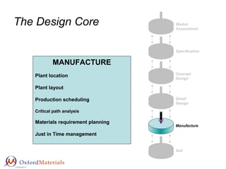
1. The Design Core Market
Assessment
Specification
Concept
Design
Detail
Design
Manufacture
Sell
MANUFACTURE
Plant location
Plant layout
Production scheduling
Critical path analysis
Materials requirement planning
Just in Time management

2. Plant Location
Criterion Weighting
Possible Factory Location
A B C D E
PROXIMITYTO:
Skilled labour 7 2 14 3 21 0 0 1 7 4 28
A pool of unskilled labour 8 5 40 2 16 0 0 4 32 2 16
A motorway 7 3 21 2 14 1 7 3 21 4 28
An airport 4 1 4 3 12 4 16 2 8 2 8
The sea / a river 0 2 0 5 0 5 0 2 0 1 0
Housing 5 4 20 3 15 0 0 3 15 4 20
Amenities 5 3 15 2 10 0 0 2 10 3 15
Potential for expansion 7 2 14 1 7 5 35 3 21 2 14
Availability of grants/incentives 8 1 8 2 16 5 40 1 8 3 24
Safety 2 3 6 2 4 5 10 2 4 2 4
Planning constraints 5 2 10 3 15 5 25 4 20 2 10
Environmental impact 4 3 12 2 8 4 16 1 4 2 8
TOTAL 164 138 149 150 175

3. ‘Functional’ Plant Layout
L L
L L
M M
M M
D D
D D
G G
G G
ASSEMBLY
1
ASSEMBLY
2
Product 2
Material 2
Material 1
Product 1
• Common for a large variety of
products in batch volumes.
• Similar processes are grouped
together.
• Inefficient: Long material transport
routes from dept. to dept. Work in
progress is high. Tracking of orders
can be difficult.
• Advantages: Specialist labour and
supervision. Flexibility as material
can be rerouted in any sequence.

4. ‘Product’ Plant Layout
A
S
S
E
M
B
L
Y
L M D G
L M D G
L M D G
• Mass production where variety is small
and production volumes are very high.
• AKA ‘flow’ or ‘line’ layout.
• More efficient, but less flexible than
‘functional’ layout.
• Work in progress is minimised, and jobs
are easily tracked.
• Investment in specialised capital
equipment is high, so a reliable and steady
demand is required.
• Very sensitive to machine breakdown or
disruption to material supply.

5. ‘Cellular’ Plant Layout
L M
D G
M M
D G
L L
L G
ASSEMBLY
CELL 3
ASSEMBLY
CELL 2
ASSEMBLY
CELL 1
• AKA ‘Group Technology’
• Each cell manufactures products
belonging to a single family.
• Cells are autonomous manufacturing
units which can produce finished parts.
• Commonly applied to machined parts.
• Often single operators supervising CNC
machines in a cell, with robots for
materials handling.
• Productivity and quality maximised.
Throughput times and work in progress
kept to a minimum.
• Flexible.
• Suited to products in batches and where
design changes often occur.

6. Designing a ‘Cellular’ Layout
Part Route Part Route
1
2
3
4
5
6
7
8
L1,L2,M1,D1,G1,F
L1,M1,D1,G2,F
L2,M1,D1,M2,G1
L2,D1,M1,M2,G2,G1
L1,L2,M2,G1,D2,G2
L2,M1,D1,G2,G1
L1,M1,D1,G1,D1,G1,F
L2,D2,G1,D2,G1,G2
9
10
11
12
13
14
15
16
L3,M1,G2,M1,D1,G2
L2,L3,M1,G1,G2,F
L2,M1,G1,M1,G2,F
L1,L2,M1,D1,M2,G1
L1,L3,M1,D1,G2,F
L3,M1,G1,M1,G1,G2,F
L1,M2,D2,G1,G2
L1,M1,D1,M2,G1,F
A company produces 16 specialist tools.
The company is planning to relocate and reorganise production with a ‘cellular’ layout, with
cells containing 5-7 machines each.
Production involves 10 types of machine: L1, L2, L3, D1, D2, M1, M2, G1, G2, F.
4 machines of each type are used, except D2 of which there is only 1.
First draw up a table of part
routes.

7. Designing a ‘Cellular’ Layout
Part
Machine
L1 L2 L3 D1 D2 M1 M2 G1 G2 F
1
2
3
4
5
6
7
8
9
10
11
12
13
14
15
16
1
1
1
1
1
1
1
1
1
1
1
1
1
1
1
1
1
1
1
1
1
1
1
1
1
1
1
1
1
1
1
1
1
1
1
1
1
1
1
1
1
1
1
1
1
1
1
1
1
1
1
1
1
1
1
1
1
1
1
1
1
1
1
1
1
1
1
1
1
1
1
1
1
1
1
1
1
1
1
1
1
1
1
1
1
Draw-up a machine-part incidence matrix
∑=
−=
n
j
qjpjpq aad
1
a=1 used
a=0 not used
‘Proximity’ between machines
e.g. p=1, q=2 then d12=3 (L2,G1,G2) 0
2
4
6
8
1 7 16 12 3 4 6 2 13 9 10 11 14 8 5 15
‘Proximity’ between
machines/clusters
Construct a dendrogram based on pairs
of closely related machine routes

8. Designing a ‘Cellular’ Layout
L1 L2 M1
D1
M2G1F
Cell A
Routes 1, 7, 16
M1L2L1
D1
M2G2G1
Cell B
Routes 12, 3, 4, 6
L1 L3
M1
D1G2F
Cell C
Routes 2, 13, 9
L2 L3
M1
G1G2F
Cell D
Routes 10, 11, 14
M2L2
L1
D2
G2G1
Cell E
Routes 8, 5, 15
88
8 8
8
8
Machine No. before No. after
L1
L2
L3
D1
D2
M1
M2
G1
G2
F
4
4
4
4
1
4
4
4
4
4
4
4
2
3
1
4
3
4
4
3
Total 37 32

9. Other Plant Layouts
PRODUCT
MATERIAL
MATERIAL
LABOUR
LABOUR
COMPONENTS
COMPONENTS
‘Fixed Position’ Layout (right)
• Single large, high cost components or
products.
• Product is static. Labour, tools and
equipment come to the work rather than
vice versa.
‘Random’ Layout
• Very inefficient
• Small factories, start-up companies.
‘Process’ Layout
• Process industries, e.g. steelmaking.
• The process determines layout.

10. Single Machine Scheduling
A CB
Schedule ABC
2 6 7
I.
Time
AC B
Schedule CAB
1 3 7
II.
Time
Shortest Processing Time (SPT)
Henry L. Gantt, Frankford Arsenal, USA
Average customer waiting time:
I. (3+7+8)/3 = 6 h
II. (2+4+8)/3 = 4 2
/3 h
⇒ Shortest jobs before longer jobs
+ 1 h delivery time to customer
Others
Minimise average
processing time
WSPT Schedule in order of
weighted shortest processing
time
Minimise average delay
EDD Schedule in order of
earliest due date
WEDD Schedule in order of
weighted earliest due date

11. Scheduling Operations in Series
Schedule ABCDE
6 13 25
Time
2317
A B C D E
6 13 25 2819
A B C D E
11 32
Prep.
Phot.
Sample: A B C D E
Time to
prepare (h)
Time to
photograph (h)
6 7 4 6 2
5 6 6 3 4
Johnson’s Algorithm
Step 1. Find next job with the
shortest processing time on either
machine.
Step 2. If on 1st machine then
schedule at next earliest position.
Step 3. If on 2nd machine then
schedule at next latest position.
A
A
B
B
C
C
D
D
E
E
Prep.
Phot.
6 13 252 19
ABC DE
6 24 2819
ABC DE
122
Prep.
Phot.

12. Scheduling Machines in Parallel
A
B
C
D
E
F
G
H
I
J
K
L
M
Machine 1
Machine 2
Machine 3
Time
A
A
31
C
C
25
K K
46
J
J
45
F
F
43
G G
28
Greedy heuristic: Biggest job first.
Schedule next longest job
on next available machine
31
5
25
7
10
12
28
6
12
17
21
4
8
I
I
55
E
E
55
M
M
54
D
61
H
H
D
61
B
B
60
L
L
64

13. Critical Path Analysis
Operation
Time
Required
(h)
Predecessors Earliest finish time of
predecessors
Earliest
Start
A
B
C
D
E
F
G
H
I
J
K
3
3
1
2
8
4
1
4
12
6
4
-
A
-
C
A, D
-
F
-
C
B, E, G
H, I, J
-
3(A)
-
1(C)
3(A), 1+2(D)
-
4(F)
-
1(C)
3+3B, 3+8(E), 4+1(G)
4(H), 1+12(I), 11+6(J)
0
3
0
1
3
0
4
0
1
11
17
More complex scheduling involving operations in parallel and in series

14. Critical Path Analysis
K
17 21
4
C
0 1
1
A
0 3
3
F
0 10
4
G
4 11
1
E
3 11
8
B
3 11
3
D
1 3
2
I
1 17
12
H
0 17
4
J
11 17
6
Time (h)8 16
A
B
C
D
E
F
H
I
G
J
K
Operation period
Allowable slack
Critical path
K
17 21
4
C
0 1
1
A
0 3
3
E
3 11
8
D
1 3
2
J
11 17
6
Earliest
start time
Latest
finish time
Operation
time

15. Materials Requirement Planning (MRP)
MATERIALS REQUIREMENTS PLANNING PROGRAM
Bill of
Materials
Current
Inventory
Purchasing
Schedule
Material
Control
Schedule
Manufacturing
Schedule
Master
Production
Schedule

16. Master Production Schedule (MPS)
Week 5 6 7 8 9 10
Product P65 10 0 20 0 20 0
Product K92 15 20 20 25 15 20
Product U37 30 35 5 45 30 30
41 42
20 0
20 20
30 30
A production plan showing period by period anticipated production of finished items
N.B. It is not a sales forecast, though expected sales are a consideration
MPS is updated in a rolling fashion: adding one or more periods
to the far end of the production schedule as well as updating the
amounts to be produced
Current week
Planning period depends on
manufacturing lead time etc.

17. Master Production Schedule (MPS)
Week 5 6 7 8 9 10
Forecast
demand
10 10 10 10 10 10
MPS 10 0 20 0 20 0
Orders
accepted
8 8 5 0 2 0
Available to
promise
4 0 15 0 18 0
41 42
10 10
20 0
0 0
20 0
Product P65
Current stock on hand = 10 Current week: 4
(Current stock + MPS) – (Total orders to next production run) = Stock available to promise
10 10 8 8 4+ - + =

18. Master Requirements Planning (MRP)
Week 1 2 3 4 5 6
Gross
requirements
10 20 10 30 0 10
Scheduled
receipts
10 25
Net
requirements
25 10
Planned order
receipts
35
Planned order
releases
35
Projected
inventory
10 10 15 5 10 10 0
37 38
20 20
20 20
40
20 0
Product P65
Current stock on hand = 10
Planning
period

19. Economic Order Quantity
Time
Inventorylevel
Order
Arrives
Q
Let
C0 = Cost of placing an order,
CH = Cost (per year) of holding a single unit in stock
D = Demand rate (no. units per year)
No. orders per year = D/Q
Total cost of ordering stock per year = COD/Q
Holding cost per year is CH x Q/2 (average stock level)
Total cost per year,
To minimize cost set
So the economic order quantity,
For a given continuous demand rate,
inventory can be controlled with large
order sizes Q ordered at low
frequencies or small order sizes
ordered at high frequencies. What is
the optimum value of Q = Q* ?
2
QC
Q
DC
T HO
+=
0
2d
d
2
=+−= HO C
Q
DC
Q
T
2/1
2
* 





=
H
O
C
DC
Q

20. Economic Order Quantity
The flat minimum phenomenon
Q
Totalcostperyear,T
Holding costs alone
2
QC
Q
DC
T HO
+=
Demand is never truly predictable.
What happens if we get the value of Q slightly
wrong?
Suppose that instead of ordering Q*, we
order an amount )1(* δ+= QQ
2
)1(*
)1(*
δ
δ
+
+
+
=
QC
Q
DC
T HO
)2/1()2( 22/1
δ+≈ HOCDCTSo,
Even if we over-order by 10%, the cost of
the stock is only increased by about 0.5%.
)1...1(
2
1
1
1
2
2
2
)1(
2)1(
32
2/1
2/1
2/12/1
δδδδ
δ
δ
δ
δ
++−+−





=




++
+






=





+
+





+
=
HO
HO
H
OH
O
HO
CDC
CDC
C
DCC
DC
CDC

21. Just in Time Manufacture (JIT)
• Reduction of batch sizes
Large batch sizes are costly to produce (large amounts of stock, long time to
produce the whole batch before reaping a return). JIT philosophy is to reduce
batch sizes towards unity.
• Reduction of set-up times
Each batch is costly in set-up time. Achieving small batch sizes requires the strive
towards reduced set-up times. Achieved with, e.g. reprogrammable equipment,
quick change tooling, storage of tooling close to machine etc.
• Reduction of buffer inventories
Materials, sub assemblies, part processed parts etc. in queues/storage are costly
and inefficient. They cost money rather than make money.
• Frequent deliveries and long term relationships with suppliers
Reduced batch sizes and buffer inventories require small, but frequent deliveries
often on demand. Suppliers viewed as partners rather than adversaries.
A system of organising manufacturing, the essence of which is to remove
waste, particularly in the waste of time and resources associated with stocks
held at different stages of the manufacturing process.

22. Just in Time Manufacture (JIT)
• Short lead times
Results in increased responsiveness to customer requirements and therefore
increased competitiveness.
• Simple material flows and reduced floor space
‘Product’ or ‘cellular’ plant layouts are essential to ensure smooth flow of material
through the factory. The ‘functional’ layout results in too much work in progress.
• Teamwork and a motivated workforce
The sensitivity of the system to down-time requires that problems are solved
quickly, and by all concerned. Problem solving and continual improvement cannot
be achieved without consultation and involvement of the workforce who are the
people on the shop floor that know the operations best.
• Workers responsible for the quality of their own work
Workers on the shop floor should think of themselves as making parts rather than
just operating a machine. ‘Non-productive’ costs such as education of the
workforce should be viewed as necessary.
• Visibility of performance
Simple flow of material allows each member of the workforce to see how their work
fits into the rest of the factory, and therefore allows rapid problem solving.

23. Material Control in JIT: Kanban
• Nothing can be made without an authorizing kanban from the next process
in line.
• Kanban system ensures nothing is made that is not required, and everything
is made just in time.
• Kanbans specify the item, number to be used in each batch, stocking
locations, the material required and where to find it.
• Production-kanbans move with the parts as they are processed, with a
different production-kanban for each operation.
• Move-kanbans remain between one workstation and the next.
• In both cases there is a well defined quantity of parts referred to that are
kept in a container holding exactly that number.
Kanban
A card or docket that authorizes either processing of a part at a particular
workstation, or movement of parts between workstations.

24. A Kanban System
M
P M
P
P M
M
P P
Workstation
A
Workstation
B
P
Containers waiting
to be moved to
workstation B
Parts waiting to
be processed at
workstation B
Kanban authorizing
production at workstation A
Kanban authorizing move from
workstation A to workstation B
Production transaction
Move transaction

25. The Kanban System
• The amount of inventory in the system is determined by the number of kanbans.
• If demand stops suddenly then production continues until every kanban is attached to
a full container. Represents the maximum amount of inventory possible.
• If a reduction in inventory of the system is required then it is achieved by simply
reducing the number of kanbans.
• Kanban system is highly visible. No need for extensive computation to track
requirements in the factory.
• Only works well for repetitive production, and for a relatively stable level of demand.
• Kanban is a ‘pull system’ where parts are only processed at one workstation when
there is a requirement from the following workstation. In a ‘push system’ parts are
continued to be processed at workstation A whether or not they are required at
workstation B. If they are not required at B, e.g. due to machine failure, then parts
processed at A queue up to be processed at B and inventory levels rise unnecessarily
and control of inventory becomes difficult. However, in the kanban system if one
workstation fails then authorization for movement to that workstation stops and the
whole process comes to a halt. The system therefore demands strict discipline in
maintenance.

26. The Design Core Market
Assessment
Specification
Concept
Design
Detail
Design
Manufacture
Sell
SELL
That’s another story!