Bituminous mix design

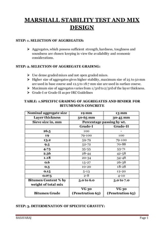
1. BASAVARAJ Page 1
MARSHALL STABILITY TEST AND MIX
DESIGN
STEP: 1. SELECTION OF AGGREGATES:
 Aggregates, which possess sufficient strength, hardness, toughness and
soundness are chosen keeping in view the availability and economic
considerations.
STEP: 2. SELECTION OF AGGREGATE GRADING:
 Use dense graded mixes and not open graded mixes.
 Higher size of aggregates gives higher stability, maximum size of 25 to 50 mm
are used in base course and 12.5 to 18.7 mm size are used in surface course.
 Maximum size of aggregates varies from 1/3rd to2/3rd of the layer thickness.
 Grade‐I or Grade‐II as per IRC Guidelines
TABLE: 1.SPECIFIC GRADING OF AGGREGATES AND BINDER FOR
BITUMINOUS CONCRETE
STEP: 3. DETERMINATION OF SPECIFIC GRAVITY:
Nominal aggregate size 19 mm 13 mm
Layer thickness 50-65 mm 30-45 mm
Sieve size in, mm Percentage passing by wt.
Grade-I Grade-II
26.5 100 -
19 79-100 100
13.2 59-79 79-100
9.5 52-72 70-88
4.75 35-55 53-71
2.36 28-44 42-58
1.18 20-34 34-48
0.6 15-27 26-38
0.3 10-20 18-28
0.15 5-13 12-20
0.075 2-8 4-10
Bitumen Content % by
weight of total mix
5.0 to 6.0 5.0 to 7.0
Bitumen Grade
VG 30
(Penetration 65)
VG 30
(Penetration 65)

2. BASAVARAJ Page 2
 Determine the of Specific Gravity of Aggregates and Bituminous Material
STEP: 4. PROPORTIONING OF AGGREGATES: (ANALYTICAL METHOD)
After selecting the aggregates and their gradation, proportioning of aggregates has to
be done and following are the common methods of proportioning of aggregates:
1. Trial and error procedure: Vary the proportion of materials until the
required aggregate gradation is achieved.
2. Graphical Methods: Twographical methods in common use for
proportioning of aggregates are, Triangular chart method and Rothfutch’s
method. The former is used when only three materials are to be mixed.
3. Analytical Method: In this method a system of equations are developed
based on the gradation of each aggregates, required gradation, and solved by
numerical methods. With the advent of computer, this method is becoming
popular and is discussed below. The resulting solution gives the proportion of
each type of material required for the given aggregate gradation.
GRADATION BY ANALYTICAL METHOD USING EXCEL-SOLVER
A dense mixture may be obtained when this particle size distribution follows Fuller law
which is expressed as:
P=100 x (𝒅/𝑫) 𝒏
Where, P= is the percent by weightofthe total
mixture passing any given sieve sized,
d=is sieve size in mm
D=is the size of the largest particlein that
mixture in mm
n= parameter depending on the shape ofthe aggregate(0.5
for rounded aggregates).
Based on this law Fuller-Thompson gradation charts were developed by adjusting the
parameter n for fineness or coarseness of aggregates. Practical considerations like
construction, layer thickness, workability, etc. are also considered. For example Table: 1
provides a typical gradation for bituminous
Concrete for a thickness of 40 mm.
The gradation required for a typical mix is given in Table: 2.in column and 2. The
gradation of available for three types of aggregate A, B, and C is given in column 3, 4, and
5. Determine the proportions of A, B and C if mixed will get the required gradation in
column 2.
TABLE: 2.GRADATION

3. BASAVARAJ Page 3
Sieve
Size
in (mm)
(1)
Required
Gradation
Range
(2)
Filler
Material
(A)
(3)
Fine-
Aggregate
(B)
(4)
Coarse -
Aggregate
(C)
(5)
26.5 100 100 100 100
19 100 100 100 100
13.2 79-100 100 100 84
9.5 70-88 100 100 71
4.75 53-71 100 100 50
2.36 42-58 100 71 36
1.18 34-48 100 50 25
0.6 26-38 100 35 20
0.3 18-28 100 25 13
0.15 12--20 71 18 9
0.075 4--10 40 13 5
The solution is obtained by constructing a set of equations considering the lower
and upper limits of the required gradation as well as the percentage passing of each type of
aggregate. The decision need to take is the proportion of aggregate A, B, C need to be
blended to get the gradation of column 2. Let x, y, and z represent the proportion of A, B,
and C respectively. Equation of the form ax + by + cz >= pl or <= pu can be written for
each sieve size, where a, b, and c are the proportion of aggregates A, B, and C passing for
that sieve size and pl and pu are the required gradation for that sieve size. This will lead to
the following system of equations:
Subjected to: x+ y + z = 1
Constraints: x + y + 0.840z ≥ 0.790
x + y + 0.710z ≤ 1.000
x + y + 0.710z ≥ 0.700
x + y + 0.710z ≤ 0.880
x + y + 0.500z ≥ 0.530
x + y + 0.500z ≤ 0.710
x + 0.710y + 0.360z ≥ 0.420
x + 0.710y +0.360z ≤ 0.580
x + 0.500y + 0.250z ≥ 0.340
x + 0.500y + 0.250z ≤ 0.480
x + 0.350y + 0.200z ≥ 0.260
x + 0.350y + 0.200z ≤ 0.380
x + 0.250y + 0.130z ≥ 0.180

4. BASAVARAJ Page 4
x + 0.250y + 0.130z ≤ 0.280
x + 0.180y + 0.090z ≥ 0.120
0.710x + 0.180y+ 0.090z ≤ 0.200
0.400x + 0.130y + 0.050z ≥ 0.040
0.400x + 0.130y + 0.050z ≤ 0.100
Solving the above system of equations manually is extremely difficult. Good computer
programs are required to solve this. Software like solver in Excel can be used. Soving
this set of equations is outside the scope of this book. Suppose the solution to this problem
is x = 0.06, y = 0.36, and
z = 0.58. Then Table: 3.Shows how when these proportions of aggregates A, B, and C are
combined, produces the required gradation.
TABLE: 3.RESULT OF MIX DESIGN
Sieve
Size
in (mm)
(1)
Required
Gradation
Range
(2)
Filler
Material
(A)
(3)
Fine-
Aggregate
(B)
(4)
Coarse -
Aggregate
(C)
(5)
Combined
Gradation
Obtained
(6)
26.500 100.000 6.074 35.926 58.000 100.000
19.000 100.000 6.074 35.926 58.000 100.000
13.200 79-100 6.074 35.926 48.720 90.720
9.500 70-88 6.074 35.926 41.180 83.180
4.750 53-71 6.074 35.926 29.000 71.000
2.360 42-58 6.074 25.508 20.880 52.462
1.180 34-48 6.074 17.963 14.500 38.537
0.600 26-38 6.074 12.574 11.600 30.248
0.300 18-28 6.074 8.982 7.540 22.596
0.150 12-20 4.313 6.467 5.220 15.999
0.075 4-10 2.430 4.670 2.900 10.000
STEP: 5. PREPARATION OF SPECIMEN:
 The preparation of specimen depends on the stability test method employed.
 The stability test methods, which are in common use for the design mix, are,
Marshall, Hubbard‐ Field and Hveem.
 Hence the size of specimen, compaction and other specifications should be
followed as specified in the stability test method.

5. BASAVARAJ Page 5
PREPARATION & STABILITY TEST BY MARSHALL METHOD:
 Stability of the bituminous mix specimen is defined as a maximum load carried
in kg at the standard test temperature of 60 ̊C when load is applied under
specified test conditions.
 Flow Value is the total deformation that the Marshall test specimen undergoes
at the maximum load expressed in mm units.
 In this test an attempt is made to obtain optimum binder content for the
aggregate mix.
 There are twomajor features of the Marshall method of designing mixes
namely,
1) Density – void analysis
2) Stability – flow test
THE SPECIFICATIONS OF APPARATUS:
 Cylindrical mould, 101.6 mm diameter and 63.5 mm height.
 Base plate and collar.
 A compaction pedestal and hammer are used to compact.
 Sample extractor is used to extrude the compacted specimen from the mould.
 A breaking head is used to test the specimen by applying a load on its periphery
perpendicular to its axis in a loading machine at a rate of 50 mm per
minute.(50mm/min)
 A dial gauge fixed to the guide rods of the testing machine serves as flow meter
to measure the deformation of the specimen during loading.
MARSHALL STABILITY TEST MACHINE

6. BASAVARAJ Page 6
Fig:BREKING HEAD Fig:MOULD WITH COLLAR
TEST PROCEDURE:
1. The coarse aggregates, fine aggregates and the filler material are proportioned
and mixed in a such way that final gradation of the mixture is within the range
specified for the type of bituminous mix.
2. Approximately 1200 gm. of the mixed aggregates and the filler are taken and
heated to a temperature of 175 to 190 ̊C.
3. The bitumen is heated to a temperature of 121 to145 ̊C.
4. The required quantity of the first trial percentage of bitumen (say, 3.5 or 4.0
percent by weight of aggregates) is added to the heated aggregates.
5. It is thoroughly mixed at the desired temperature of 154 to 160 ̊C.
6. The mix is placed in a pre‐heated mould and compacted by a rammer (4.54 kg)
with 75 blows on either side at temperature of 138to 149 ̊C
7. Three or four specimens may be prepared using each trial bitumen content.
8. The compacted specimens are cooled to room temperature in the mould and
then removed from the molds using a specimen extractor.
9. The diameter and mean height of the specimen are measured.
10. The weight of each specimen in air and suspended in water is determined.
11.The specimens are kept immersed in water in a thermostatically controlled
water bath at 60 ± 10 ̊C for 30 to 40 minutes.
12.The specimens are taken out one by one.
13.The specimen is placed in the Marshall Test head.
14.It is then tested to determine Marshall Stability Value which is the maximum
load before failure and the Flow value which is the deformation of the specimen
up to the maximum load.
15.The corrected Marshall Stability value of each specimen is determined by
multiplying the proving ring reading with its constant.
16.If the average thickness of the specimen is not exactly 63.5 mm, a suitable
correction factor is applied.
17.The above procedure is repeated on specimens prepared with other values of
bitumen contents in suitable increments; say 0.5 percent, up to about 7.5 or
8.0 percent.

7. BASAVARAJ Page 7
18.If the average thickness of the specimen is not exactly 63.5 mm, a suitable
correction factor is applied.
CALCULATIONS:
I. DENSITY AND VOID ANALYSIS:
i. Voids in Mineral Aggregates (VMA):
VMA =Vv + Vb
Where, Vv =Volume of air voids in compacted mass
Vb =Volume of the bitumen in compacted mass
ii. Voids Filled with Bitumen (VFB):
VFB in percentage =
𝐕𝐛
𝐕𝐌𝐀
x 100
VFB in percentage =
𝐕𝐛
𝐕𝐯+𝐕𝐛
x 100
II. SPECIFIC GRAVITY:
i. Bulk Specific Gravity of Bituminous mix(Gb):
Gb =
𝐖𝐞𝐢𝐠𝐡𝐭 𝐢𝐧 𝐀𝐢𝐫
𝐖𝐞𝐢𝐠𝐡𝐭 𝐢𝐧 𝐚𝐢𝐫−𝐖𝐞𝐢𝐠𝐡𝐭 𝐢𝐧 𝐖𝐚𝐭𝐞𝐫
ii. Theoretical Specific Gravity of Bituminous mix(Gt):
Gt =
𝟏𝟎𝟎
𝐖𝟏
𝐆𝟏
+
𝐖𝟐
𝐆𝟐
+
𝐖𝟑
𝐆𝟑
+
𝐖𝟒
𝐆𝟒
Where, G1, G2, G3, G4 are apparent specific gravity of coarse aggregates, fine
aggregate, filler,and bituminous binder respectively.
Where, W1, W2, W3, W4 are percent by weight of coarse aggregate, fine
aggregate, filler and bituminous binder respectively.
III. VOLUME:
i. Volume of Air Voids (Vv):
Vv =
𝐆𝐭−𝐆𝐛
𝐆𝐭
x100
ii. Volume of Bitumen (Vb):
Vb =
𝐖𝟒
𝐆𝟒
x Gb

8. BASAVARAJ Page 8
GRAPH:
 The average value of each of the above properties are found for each mix with the
different bitumen content
 Graphs are plotted with the bitumen content on the X-axis and the following values
on Y-axis.
1. Marshall Stability Value.
2. Flow Value.
3. Unit Weight.
4. Percentage Voids in total mix.(Vv)
5. Percentage Voids Filled with Bitumen(VFB)
OPTIMUM BITUMEN CONTENT (OBC)
The optimum bitumen content (OBC) for the mix design is found by taking the
average value of the following three bitumen contents found from the graphs of the rest
results.
1. Bitumen content corresponding to maximum stability.
2. Bitumen content corresponding to maximum unit weight.
3. Bitumen content corresponding to the median of designed limits of percent
air voids in total mix (5%)
The Marshall Stability value, Flow value and percent voids filled with Bitumen at
the average value of bitumen content are checked with the Marshall Stability design
criteria/specification.
DESIRED VALUES:
TABLE: REQUIREMENT FOR BITUMEN CONCRETE LAYERS
(TABLE 500-19,MoRTH,2001)
Minimum Stability (kN at 60 ̊C ) 9.0
Minimum Flow (mm) 2
Maximum Flow (mm) 4
Compaction level (No.of blows) 75 blows on each of two faces of the
specimen
Percent air voids 3-6
Percent voids in mineral
aggregate(VMA)
See Table No.
Percent voids filled with
bitumen(VFB)
65-75
Loss of stability on immersion in
water at 60 ̊C (ASTMD 1075)
Min.75 % retained strength

9. BASAVARAJ Page 9
TABLE: MINIMUM PERCENT OF VOIDS IN MINERAL AGGREGATE
(VMA)
BITUMINOUS CONCRETE (TABLE 500-12, MoRTH, 2001)
Nominal
Maximum
Particle size in
mm
Minimum VMA percent related to Design Air Voids, percent
3.0 4.0 5.0
9.5 14.0 15.0 16.0
12.5 13.0 14.0 15.0
19.0 12.0 13.0 14.0
25.0 11.0 12.0 13.0
37.5 10.0 11.0 12.0